06 Modeling
Introduction
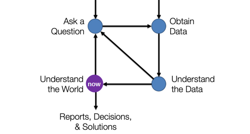
- Understand the World: starting machine learning
Model : idealized representation of a system
not exact nor correct (approximated but accurate enough)
- Why do we build Models?
- To understand complex phenomena occuring in the world we live in
- simple and interpretable
physics velocity, acceleration
- simple and interpretable
- To make accurate predictions about unseen data
-
predicting email is spam/not - black-box models: making extremely accurate predictions but uninterpretable model
-
- To understand complex phenomena occuring in the world we live in
- Learning from DATA
- no analytic solution (or hard to get) but have data \(\Rightarrow\) use Data!
- no need to do everything my mathematical modeling
Example: Recommendation Systems
- `20%` sales from recommendation (Amazon)
- `10%` improvement = 1 million dollar prize (Netflix)
- power of learning from data: entire process can be automated without having to look at video content or viewer taste
Dall-E2,ChatGPTall based on Data- The essence of learning from data
- We have data
- A pattern exists therin
- We cannot pin it down analyticall (or is challenging)
Notations
- \(y\) : true observations (Ground Truth)
- \(\hat{y}\) : predicted observations
- \(\theta\) : parameter(s) of model (what we are trying to estimate)
- not all models have parameters
ex: KDE
- not all models have parameters
\(\hat{\theta}\) : fitted/optimal parameter(s) we solve for \(\Leftarrow\) goal (Final Parameter)
- \(tune \theta\) to minimize \(y\) and \(\hat{y}\)
Constant Model
\[\hat{y} = \theta\]Constant Model : ignore any relationships between variables and predict the same number for each individual (predicting constant)
- aka summary statistic (of data)
- GOAL: find \(\hat{\theta}\)
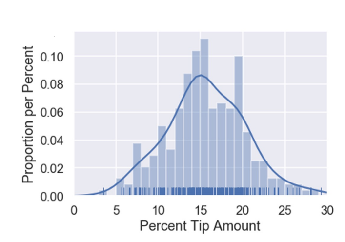
- Case Study: Tips
- model to predict some numerical quantity of population:
- percentage tip given at restaurants
- GPA of students and Korea University
- Constant model: ignoring total bill price, time of day, customers’ emotion…when predicting tips
- model to predict some numerical quantity of population:
Prediction vs Estimation
Estimation task of using data to determine model parameters Prediction task of using a model to predict output (for unseen data) ifestimates exist for model paramtersthencan use model for prediction
Loss Functions
Loss : cost of making prediction
- metric of how
goodorbadour predictions are
ifprediction \(\leftrightarrow\) actual value \(\Rightarrow\) low lossifprediction \(\longleftrightarrow\) actual value \(\Rightarrow\) high loss-
error for a single prediction: =
actual-predicted(\(y_i - \hat{y_i}\))- natural choice of loss function
BUTthis treats negative and positive predictions differently-
value = `15`; predicting `16` should equal to predicting `14` - \(\Rightarrow\) 2 natural loss functions
-
Squared Loss
\(L_2(y, \hat{y}) = (y-\hat{y})^2\)
- single data point in general = \((y-\hat{y})^2\)
constant model (since \(\hat{y}=\theta\)) = \((y_i-\theta)^2\)
ifprediction === actual observation \(\Rightarrow\)loss= 0- low loss \(\Rightarrow\) Good Fit!
Absolute Loss
\(L_1(y, \hat{y}) = |y-\hat{y}|\)
constant model \((\hat{y}=\theta ) = [y-\theta]\)
ifprediction === actual observation \(\Rightarrow\)loss= 0- low loss \(\Rightarrow\) Good Fit!
- both loss functions have drawbacks; there are more loss functions
Emprical Risk
- average loss across all points (not just a single point)
\(\frac{1}{n}\sum_{i=1}^n L(y_i, \hat{y_i})\)
- tells how well model fits the given data
- find parameter(s) minimizing the average loss
- aka emipirical risk, objective function
MSE and MAE
| MSE | Mean Squared Error | squared loss | \(MSE(y, \hat{y}) = \frac{1}{n}\sum_{i=1}^n(y_i-\hat{y_i})^2\) |
| MAE | Mean Absolute Error | absolute loss | \(MAE(y, \hat{y}) = \frac{1}{n}\sum_{i=1}^n[y_i-\hat{y_i}]\) |
MSE
- average loss typically written as a function of \(\theta\)
\(R(\theta) = \frac{1}{n}\sum_{i=1}^n(y_i-\hat{y_i})^2\) \(\rightarrow \hat{\theta} =\)
argmin= argument that minimizes the following function- in constant model (\(\hat{y} = \theta\)) \(\Rightarrow\) \(R(\theta) = \frac{1}{n}\sum_{i=1}^n(y_i-\theta)^2\)
- example: 5 observations
[20, 21, 22, 29, 33]- loss for first point (
20) \(L_2(20, \theta)=(20-\theta)^2\) - average loss across all observations : \(R(\theta) = \frac{1}{5}((20-\theta)^2+(21-\theta)^2+(22-\theta)^2+(29-\theta)^2+(33-\theta)^2)\)
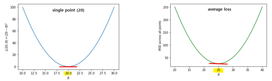
- both parabola
- loss for first observation = minimized at
20 - average loss = minimized at
25
- loss for first point (
MSE = *mean* of observations in constant models
- Proof 1 : Using Calculus
- take derivate \(\rightarrow\) set to 0 \(\rightarrow\) solve for optimizing value \(\rightarrow\) take second derivate to check convex direction (positive = upwards )
- take derivative
- \(\frac{d}{d\theta}R(\theta)\) = \(\frac{1}{n}\sum_{i=1}^n\frac{d}{d\theta}(y_i-\theta)^2\)
- = \(\frac{1}{n}\sum_{i=1}^n(-2)(y_i-\theta)\)
- = \(\frac{-2}{n}\sum_{i=1}^n(y_i-\theta)\)
- set derivate equal to 0 (find minimum point)
- 0 =\(\frac{-2}{n}\sum_{i=1}^n(y_i-\hat{y_i})\)
- 0 =\(\sum_{i=1}^n(y_i-\theta)\)
- 0=\(\sum_{i=1}^n(y_i)-n\theta\)
- \(n\theta\) = \(\sum_{i=1}^n(y_i)\)
- \(\hat{\theta}\) = \(\frac{1}{n}\sum_{i=1}^n(y_i) \Rightarrow mean\)
- take second derivative
- \(\frac{d}{d\theta}R(\theta)\) = \(\frac{-2}{n}\sum_{i=1}^n(y_i-\theta)\)
- \(\frac{d^2}{d\theta^2}R(\theta)\) = \(\frac{-2}{n}\sum_{i=1}^n(0-1)\)
- = \(\frac{2}{n}\sum_{i=1}^n(1)\) = \(2\)
- \(\Rightarrow\) positive at convex!
- Proof 2 : Using Algebraic Trick
- refresh:
- (1) sum of deviations from mean = 0 \(\sum_{i=1}^n(y_i-\hat{y})=0\)
- (2) definition of variance \(\sigma_y^2=\frac{1}{n}\sum_{i=1}^n(y_i-\hat{y})^2\)
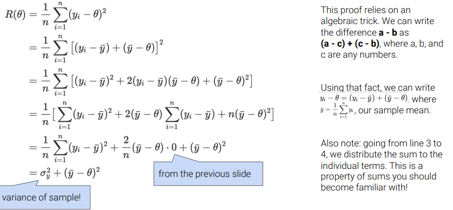
-
TBwritteninlatex later on... - \(R(\theta)\) = \(\sigma_y^2 + (\hat{y}-\theta)^2\)
- both terms = postive (variance and squared can’t be negative)
- first term does not contain \(\theta \rightarrow\) ignore
- second term contains \(\theta \rightarrow\) can be minimized (to 0) if \(\theta = \hat{y}\)
- \[\Rightarrow \hat{\theta} = \hat{y} = mean(y)\]
MAE
- mean absolute error
- example: 5 observations
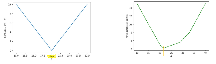
[20, 21, 22, 29, 33]- loss for first point (
20) \(L_2(20, \theta)=\mid 20-\theta \mid\) - average loss across all observations : \(R(\theta) = \frac{1}{5}(|20-\theta|+|21-\theta|+|22-\theta|+|29-\theta|+|33-\theta|)\)
- both absolute value curve
- loss for first observation = minimized at
20 - average loss = minimized at \(\approx\)
22
- results in piecewise linear function (seems to be jagged)
- seemingly not \(mean\)
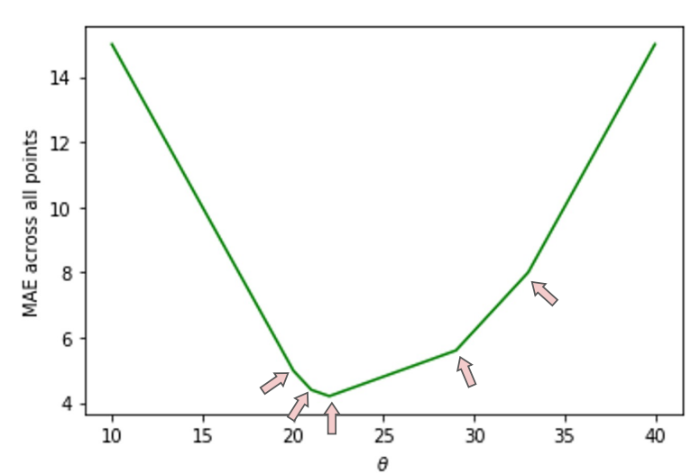
- bends (kinks) appear at observations (
[20, 21, 22, 29, 33])
- seemingly not \(mean\)
- loss for first point (
- MAE minimization using Calculus
- piecewise linear function (since it’s absolute) \(|y_i-\theta| = \begin{cases} y_i-\theta, \theta<=y_i\\ \theta-y_i, \theta>y_i \end{cases}\)
take derivative
\(\frac{d}{d\theta}\mid y_i-\theta \mid\) = \(\begin{cases} -1, \theta<=y_i\\ 1, \theta>y_i \end{cases}\)
- derivative of sum = sum of derivatives
- \(\frac{d}{d\theta}R(\theta)\)=\(\frac{1}{n}\sum_{i=1}^n \frac{d}{d\theta} \mid y_i-\theta \mid\)
- = \(\frac{1}{n}[\sum_{\theta<y_i}(-1)+\sum_{\theta>y_i}(1)]\)
set derivative equal to 0 (find minimum point)
- 0 = \(\frac{1}{n}[\sum_{\theta<y_i}(-1)+\sum_{\theta>y_i}(1)]\)
- 0 = \(-\sum_{\theta<y_i}(1)+\sum_{\theta>y_i}(1)\)
- \(\sum_{\theta<y_i}(1)\)=\(\sum_{\theta>y_i}(1)\) - \(\Rightarrow\) # of observations less than theta == number of observations greater than theta - \(\Rightarrow\) equal number of points on both left/right side - \(\Rightarrow \hat{\theta} = median(y)\)
- if even number of observations:
- ex:
[20, 21, 22, 29, 33, 35]\(\rightarrow\) no unique solution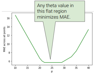
- any value in range
[22,29]minimizes MAE - usually, mean of those medians are used (
25.5)
- ex:
MSE vs MAE
- loss surface
plot of the loss encountered for each possible value of \(\theta\)
- ex:
2parameters for model \(\rightarrow\) plot =3-D
- ex:
- MSE vs MAE
| Mean Squared Error | Mean Absolute Error |
| Sample Mean | Sample Median |
| very smooth (easy to minimize) | not as smooth (kinks=not differentiable), harder to minimize |
| very sensitive to outliers | robust to outliers |
- not clear if one is better than the other (we get to choose!)
Summary
- Choose a model
- constant model (in this case) with single parameter
- Choose a loss function (\(L_2, L_1\))
- Fit the model by minimizing average loss
- choose optimal parameters to minimize average loss
- aka fitting model to the data