09 Logistic Regression
- Logistic Regression I
- Logistic Regression II
Logistic Regression I
Machine Learning Taxonomy
-
Supervised Learning (Labeled Data)
- Regression : Quantitative Response
still mostly used for classification... - Classification : Categorical Response
- Regression : Quantitative Response
- Unsupervised Learning (Unlabeled Data)
- Dimensionality Reduction
- Clustering
- Reinforcement Learning (Reward)
Alpha Go - Learning Paradigm: use of ??data to uncover an underlying process
Supervised Learning
- most studied and utilized
- training data contains explicit examples of what the ??output should be for given inputs \(\rightarrow Supervised\)
- correct label exists
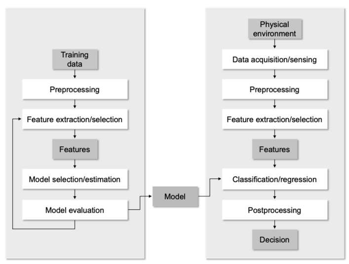
- Typical Supervised Learning Procedure
Unsupervised Learning
- no output information for training data
- instead, we get ??truth values \(\Rightarrow\) just given input examples
- Approaches:
- Clustering (K-Means, mixutre models, heirarchical)
- Hidden Markove Models (HMMs)
- Feature Extraction (PCA, iCA, SVD)
- spontaneously finding ??patterns in input data
like categorization - precursor to supervised learning
- way to create higher-level represtation of data
like automated feature extraction
Reinforcement Learning
- when training data contain no correct output for each input (no longer supervised)
- example: toddler learning not to touch a hot cup of tea
- training examples do not say what to do, still uses examples to reinforce better actions
- \(\Rightarrow\) learns what one should do in similar situations
- training example의 target ouput X, but contains
some possible output + measure of how good
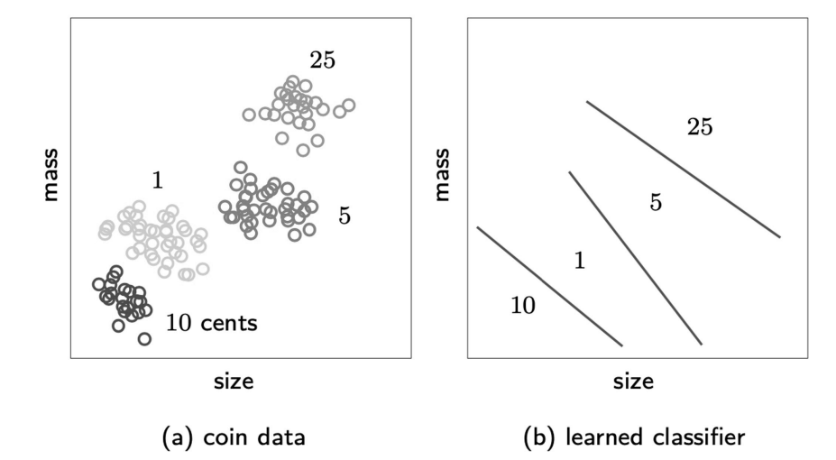
Supervised vs Unsupervised Example
- supervised
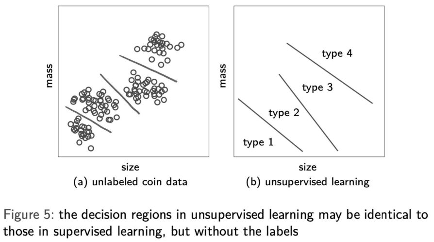
- unsupervised
Introduction
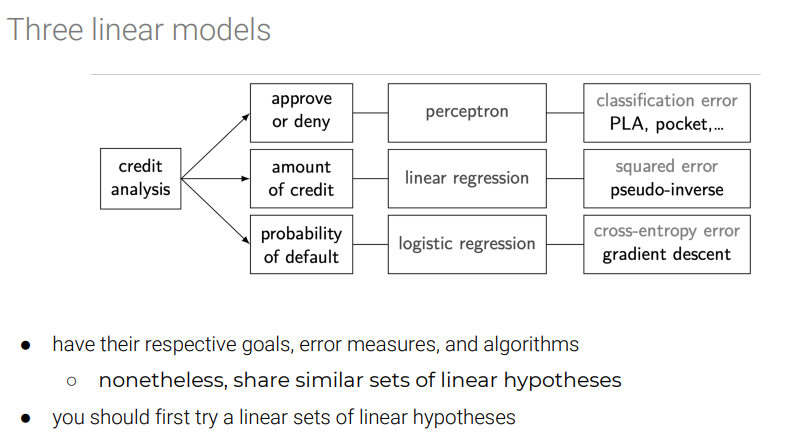
- Core of Linear Models
- signal \(s = w^Tx\) : combines input variables linearly
- Linear Regression
- \(signal = output\) for predicting real (unbounded) response
- Linear Classification
- \(signal = threshold\) at zero to preduce \(\pm 1\) output, for binary decision
- Logistic Regression aka Soft binary classification
- example: Heart attack precision
based on cholesterol lvl, blood pressure, age, weight... - 확실하게 예측은 불가능, but can predict how likely it is
- binary decision (0 or 1) 보다 더 정교 \(\rightarrow\) 0 ~ 1
closer to 1 -> more likely to get 심장마비 - \(\Rightarrow\) output:
real (like regression)but bounded (like classification) - uncertain 가능
- more appropriate than linear regression (no negative values)
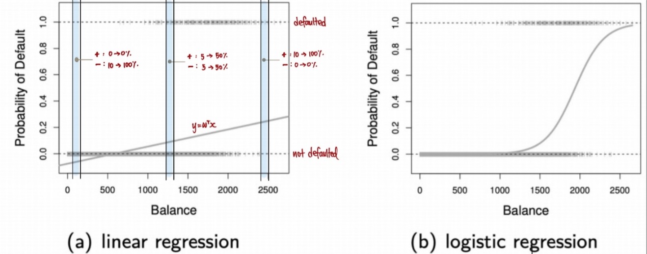
- example: Heart attack precision
Predicting Probability
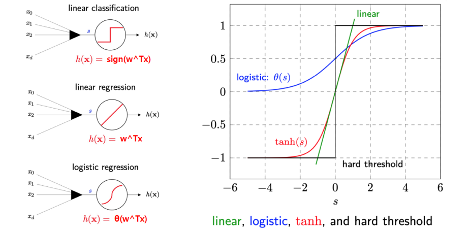
Logistic Regression Model
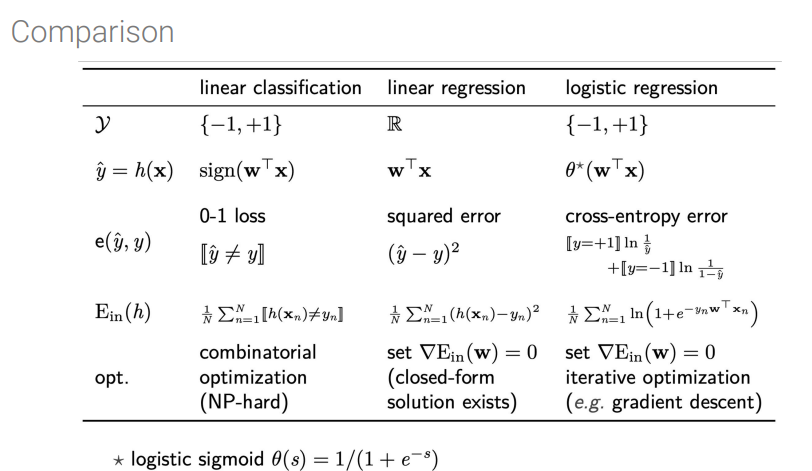
- Linear Classification: hard threshold on signal \(s=w^Tx\)
- \[h(x) = sign(w^Tx)\]
- Linear Regression: no threshold
- \[h(x) = w^Tx\]
-
Logistic Regression between linear classification & regression - \[h(x) = \theta(w^Tx)\]
- \(\theta\) : aka logistic function, Sigmoid function, soft threshold
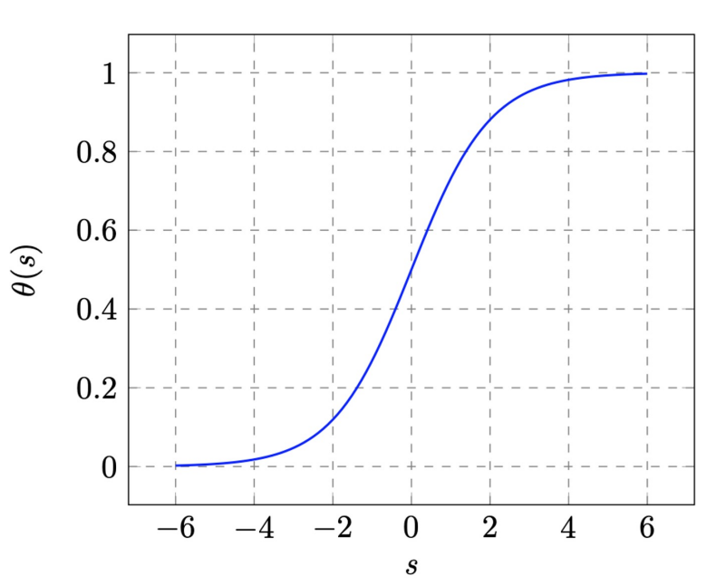
Logistic Function θ
- definition: for \(-\infty < s < \infty\) :
- \[\theta(s) = \frac{e^s}{1+e^s} = \frac{1}{1+e^{-s}}\]
Proof
- \[1-\theta(s) = 1- \frac{1}{1+e^{-s}} = \frac{e^{-s}}{1+e^{-s}} = \theta(-s)\]
- \[\theta(s) = P(+1 \mid x)\]
- \[P(-1\mid x) = 1-\theta(s) = \theta(-s)\]
output lies between 0 and 1
can be interpreted as probability for binary events \(\theta(s)\) : can define error measure, has computational advantage
Summary of Linear Models
- based on “signal” \(s = \sum_{i=1}^dw_ix_i\)
Hyperbolic Tangent (another popular sigmoid)
- \[tanh(s)=\frac{e^s-e^{-s}}{e^s+e^{-s}}\]
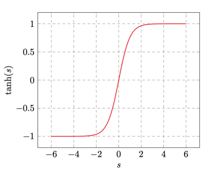
- properties- \(tanh(s)\) convergence:
- large \(\mid s\) : hard threshold
- small \(\mid s\) : no threshold
- example for heart attack:
- input x: cholesterol level, age, weight, etc..
- signal s = \(w^Tx\) : risk score
- Linear Classification: h(x) returns \(\pm 1\): heart attack (+1) or not (-1) for sure
- Linear Regression: h(x) returns risk score \(s\)
- Logistic Regression: h(x) returns \(\theta(x)\): probability of heart attack
Cross-entropy Error Measure
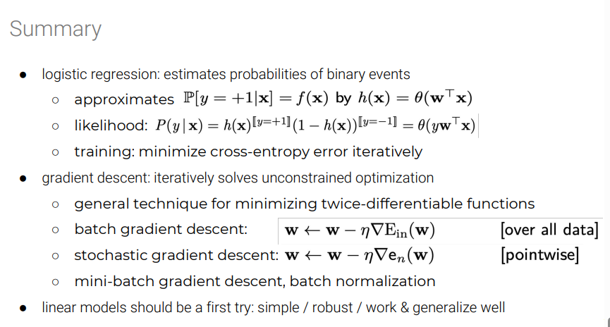
Learning Target of Logistic Reg
\[f(x) = \mathbb P [y= +1 \mid x]\]-
ex : probability of heart attack given patient characteristics - training data doesn’t give us value of \(f\), rather, gives us samples generated by this probability \((+1 / -1)\)
Fitting
-
Fitting : finiding a good \(h\)
\(h\) is good if \(\begin{cases} h(x_n) \approx 1 & y_n = +1 \\ h(x_n) \approx 0 & y_n = -1 \end{cases}\)
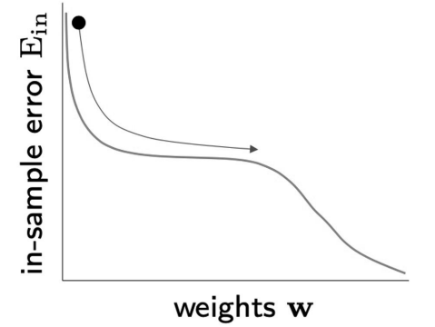
MSE works for linear models only, since it can fall into a local minimum
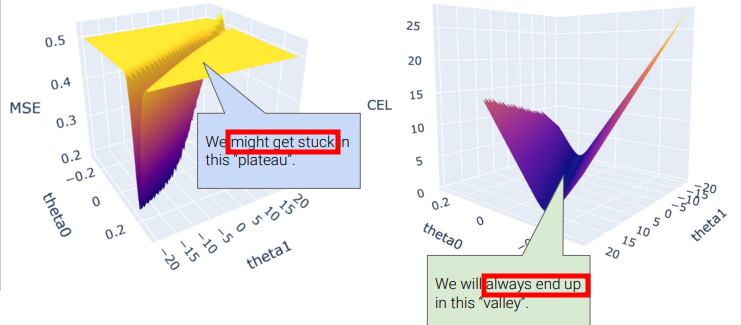
- if in the yellow area, it will get stuck and will not converge into local minimum
- \(\Rightarrow\) use
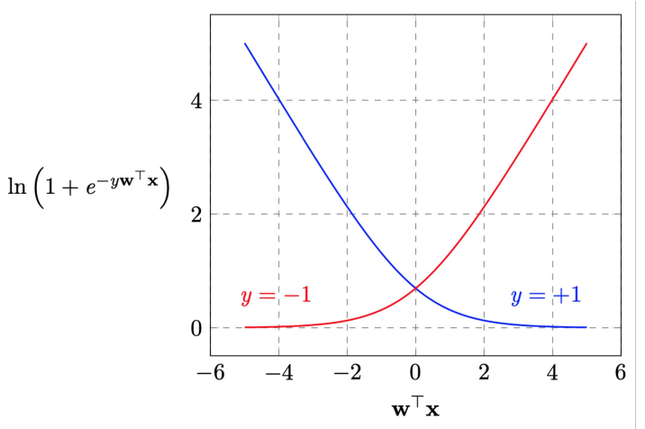
Cross-Entropy error measure
- easier to do gradient-based optimization
- \(y_n = +1\) encourages \(w^Tx_n >> 0 \longrightarrow \theta(w^Tx_n) \approx 1\) (and vice versa)
Error Measure
based on
likelihood how likely is it to get output \(y\) from input X
recall:
- \(h(x)\) = \(\theta(w^x)\)
- \(\theta(s)\) =\(\frac{e^s}{1+e^s}\)
- \(1-\theta(s)\)= \(\theta(-s)\)
PROOF
- \(P(+1 \mid x)\) = \(h(x) = \theta(w^Tx)=\frac{1}{1+exp(-w^Tx)}\)
- \(P(-1 \mid x)\) = \(1-h(x) = 1-\theta(w^Tx)\)
- 1- \(\frac{1}{1+exp(-w^Tx)}\)
- \[\frac{exp(-w^Tx)}{1+ exp(-w^Tx)}\]
- \(\Rightarrow\) \(\theta(-w^Tx)\)
Criterion for choosing h: maximum likelihood
\(\Rightarrow\) select hypothesis \(h\) that maximizes this probability
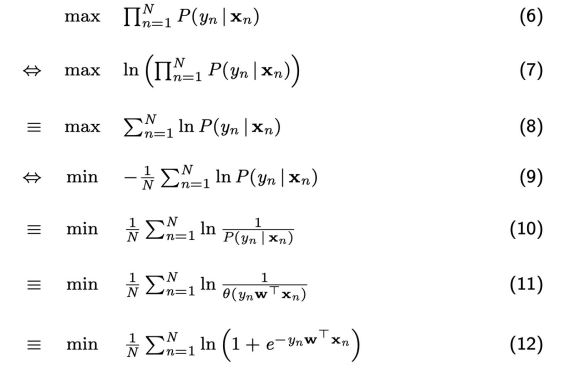
- \[P(y_1\mid x_1)P(y_1\mid x_2)\cdots P(y_N\mid x_N) \Longrightarrow \Pi_{n=1}^{N} P(y_n\mid x_n)\]
- getting all \(y_n\)’s from corresponding \(x_n\)’s
we can easily optimize/minimize if we change the maximum likelihood into log form
- \[-\frac{1}{N}ln(\Pi_{n=1}^{N} P(y_n \mid x_n)) = \frac{1}{N} \sum_{n=1}^N ln\frac{1}{P(y_n \mid x_n)}\]
- \(\Rightarrow\) negative log likelihood
- \(-\frac{1}{N}ln(\cdot)\)
= monotonically decreasing function
- \[\frac{1}{N} \sum_{n=1}^N ln\frac{1}{\theta(yw^Tx)}\]
- \[\frac{1}{N} \sum_{n=1}^N ln\begin{cases} h(x_n) & y_n = +1 \\ 1- h(x_n) & y_n = -1 \end{cases}\]
- \[\frac{1}{N} \sum_{n=1}^N {[\![ y_n = +1]\!] ln\frac{1}{h(x_n)} + [\![ y_n = -1]\!] ln\frac{1}{1-h(x_n)}}\]
- back to \(E_{in}(w) = \frac{1}{N}\sum_{n=1}^{N}ln(1+e^{y_nw^Tx_n})\)
Proof
- substituting \(\theta(yw^Tx)\), \(\frac{1}{N} \sum_{n=1}^N ln\frac{1}{\frac{e^{yw^Tx}}{1+e^{yw^Tx}}}\)
- = \(\frac{1}{N} \sum_{n=1}^N ln\frac{1+e^{yw^Tx}}{e^{yw^Tx}}\)
- = \(\frac{1}{N} \sum_{n=1}^N ln (1+e^{yw^Tx}) \cdot (e^{-yw^Tx})\)
- \[\frac{1}{N} \sum_{n=1}^N ln (1+e^{-yw^Tx})\]
- since \(e^0 = 1\)
Practice Questions
- Select the expression that describes the odds ration \(\frac{P(Y=1\mid X)}{P(Y=0\mid X)}\) of a logistic regression model. Recall: \(P(Y=0\mid X) + {P(Y=1\mid X)} = 1\) for any \(X\) and \(\theta(s) = \frac{1}{1+exp(-s)}\)
- (a) \(X^Tw\)
- (b) \(-X^Tw\)
- (c) \(exp(X^Tw)\)
- (d) \(\theta(X^Tw)\)
- (e) None of these
- Select the expression that describes \(P(Y=0\mid X)\) for a logistic regression model.
- (a) \(\theta(-X^Tw)\)
- (b) \(1-log(1+exp(X^Tw))\)
- (c) \(1+log(1+exp(X^Tw))\)
- (d) None of these
Answer
1. (c) 2. (a)- Select the expression that describes the odds ration \(\frac{P(Y=1\mid X)}{P(Y=0\mid X)}\) of a logistic regression model. Recall: \(P(Y=0\mid X) + {P(Y=1\mid X)} = 1\) for any \(X\) and \(\theta(s) = \frac{1}{1+exp(-s)}\)
Training via Gradient Descent
- update rule: \(w(t+1) = w(t) - \alpha \nabla E_{in}(w(t))\)
- \(\alpha\): learning rate (step size)
- \(E_{in}\): Training error
- examine all examples at each iteration: \(O(N)\)
- stochastic gradient descent : \(O(1)\)
- Least Mean Square (LMS) rule (Windrow-Hoff learning rule)
- when the cost function is mean squared error
- \(w\): = \(w - \alpha \nabla E_{in}(w)\)
- = \(w + \alpha (y-w^Tx)\cdot x\)
- \((y-w^Tx)\) : error
- \(x\) : input
Logistic Regression Algorithm
- intialize weights at time step t=0 to w(0)
- for t = 0,1,2…do
- \(\hspace{1cm}\)compute the gradient
- \[\nabla E_{in}(w(t)) = \frac{1}{N}\sum_{n=1}^N \frac{y_nx_n}{1+e^{y_nw^T(t)x_n}}\]
- \(\hspace{1cm}\) set the direction to move: \(v_t = - \nabla E_{in}(w(t))\)
- \(\hspace{1cm}\) update weights: \(w(t+1) = w(t) + \alpha(v_t)\)
- \(\hspace{1cm}\) iterate to next step until it is time to stop
- return final weights w
- we have to choose 2 things:
- initial weights w(0)
- criterion for stopping gradient descent
Initialization Criterion
- w(0) =
0 - works pretty well for logistic regressions
- w(0) =
random - more common, avoid getting stuck on perfectly symmetric hilltop
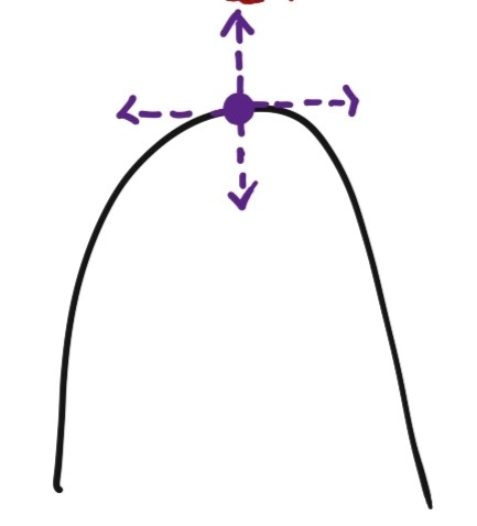
- more common, avoid getting stuck on perfectly symmetric hilltop
- choose each weight independently from normal distribution with zero mean and small variance
- used pratically
Stopping
- set
upper bound on number of iterations- PROBLEM: final weight quality not guaranteed
- check
gradient (\(\nabla E_{in}(w(t))\))under threshold whenver loss function became too small - PROBLEM: eventually must happen, but don’t know when
- PROBLEM 2: relying soley on size of gradient might stop too soon
- require
both :- (i): change in error is small
- (ii): error itself is small
- logistic regression: (1) + (2) works well
-
(1) large upper bound for number of iterations -
(2) small lower bound for the size of gradient - ultimately, (1) + (2) + (3) is good
SUMMARY
Logistic Regression II
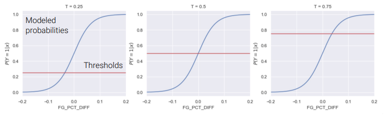
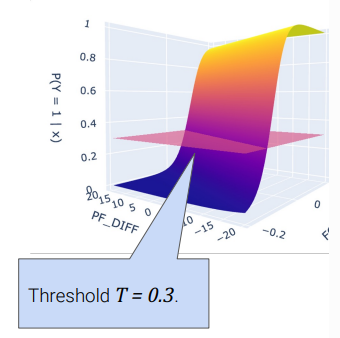
Thresholding
- outputs of Logistic Regression :
continous - Logistic Regression + Decision Rule = Classification
Decision Rule outputs 1 or 0 (depending on
threshold )- ex: \(T = 0.5\)
- \[classify(x) = \begin{cases} 1, & P(Y=1\mid x)>= 0.5 \\ 0, & P(Y=1 \mid x) < 0.5 \end{cases}\]
- widely used in object detection
Thresholds for higher dimensions: also works fine
Evaluation Metrics
Accuracy
\[accuracy = \frac{ points \hspace{0.1cm} classified \hspace{0.1cm} correctly }{ total \hspace{0.1cm} points}\]- Pitfalls of Accuracy (Spam/Ham Classification)
- 100 emails,
5 = spam,95 = ham, model classifies every email as ham - accuracy :
95%(\(\frac{95}{95+5}%\)) \(\Rightarrow\) is it good enough?NO: detecting spam email =0%
- 100 emails,
Classification Errors
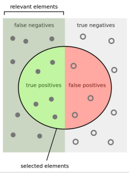
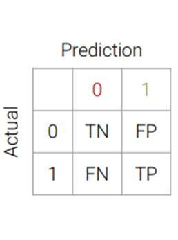
- True Positives: correctly classified as positive
- True Negatives: correctly classified as negative
- False Positives: Mistakenly detected as positive (false alarm)
- False Negatives: Failed to Detect
Precision and Recall
\[accuracy = \frac{TP + TN}{n}\]- What proportions of points did our classifier classify correctly?
- doesn’t tell full story, especially in cases with high class imbalance
- 정확도
- Of all observations that were predicted to be 1, what proportion were actually 1?
- how precise is our classifier? Penalizes false positives
- 1으로 분류된 애들 중, 실제 1인 퍼센티지
Of all observations that were actually 1, what proprtion did we predict to be one?
- How good is our classifier at detecting positives? Penalizes false negatives
- 실제로 1인 애들 중, 1으로 분류된 퍼센티지
Filtering Spam Mails:
- 100 emails,
5 = spam,95 = ham, model classifies every email as ham - \(TP = 0\) , \(FP = 0\) , \(TN=95\), \(FN=5\)
- accuracy :
95%(\(\frac{95}{95+5}%\)) - precision:
undefined(\(\frac{0}{0+0}%\)) - recall:
0%(\(\frac{0}{0+5}%\)) - \(\rightarrow\) accuracy does not tell full story
- \(\Rightarrow\) Class Imbalance: distribution of true observation is skewed (
95%of true observations are negative)
- 100 emails,
Trade-off between precision and recall
100%recall : making ALL classifier output “1”- no False Negatives, but many False Postives \(\longrightarrow\) precision low
- \(\Rightarrow\) Precision and Recall inversly related
adjusting classification threshold
-
higher threshold : \(\longrightarrow\) fewer FP, Larger Precision
-
lower threshold : \(\longrightarrow\) fewer FN, Larger Recall
-
Questions:
- In each of the following cases, what would we want to maximize: precision, recall, or accuracy?
1. Predicting whether or not a patient has some disease
- Maximize RECALL : if they are told to have disease \(\rightarrow\) further testing
- better than leaving them untreated
2. Determining whether or not someone should be sentenced to life in prison.
- Maximize PRECISION : don’t want to sentence guilty people ??????????
3. Determining if an email is spam or ham
- Maximize Accuracy : (subjective) having spam emails ending up at inbox, or hams being filter out 중 택1
Metrics
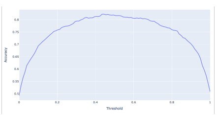
Accuracy vs. threshold
- threshold \(\uparrow\) \(\longrightarrow\) Larger FN
- threshold \(\downarrow\) \(\longrightarrow\) Larger FP
- also, accuracy is maximized doesn’t always mean \(T\) =
0.5
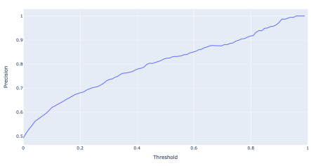
Precision vs. threshold
- threshold \(\uparrow\) \(\longrightarrow\) Fewer FP
- \(\Rightarrow\) precision increase
- \(precision\) = \(\frac{TP}{TP+FP} = \frac{TP}{predicted \hspace{0.1cm}true}\)
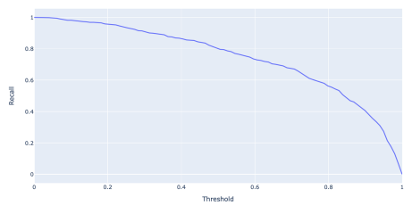
Recall vs. threshold
- threshold \(\uparrow\) \(\longrightarrow\) Larger FN
- \(\Rightarrow\) recall decrease
- \(Recall\) = \(\frac{TP}{TP+FN} = \frac{TP}{Actually \hspace{0.1cm}true}\)
Accuracy, Precision, Recall
Precision Recall Curves
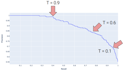
- threshold decrease: top left \(\longrightarrow\) bottom right
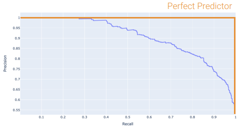
- Perfect Classifier: precision = 1, recall = 1
- PR curve to be at top right of graph
- Area Under Curve (AUC): optimal = 1
ROC more common
Other Metrics
- False Positive Rate (FPR):
- \(\frac{FP}{FP+TN} \longrightarrow\) what proportion of innocent ppl did I convict?
- True Positive Rate (TPR):
- \(\frac{TP}{TP+FN} \longrightarrow\) what proportion of guilty ppl did I convict? \(\Rightarrow\) RECALL
ROC Curves
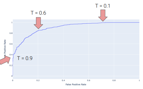
- plots
TPRvsFPR - threshold \(\uparrow\) \(\longrightarrow\)
TPR&FPRdecrease- decreased
TPR= bad (detecting fewer positives) - decreased
FPR= good (fewer false positives) - \(\Rightarrow\) Tradeoff
- decreased
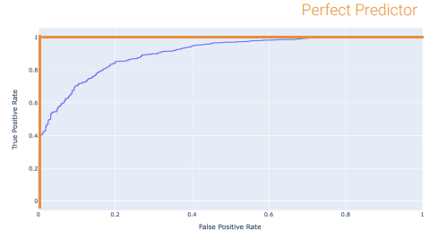
- Perfect classifier:
TPR=1,FPR= 0, top-left- best possible AUC = 1
- terrible AUC = 0.5 (randomly guessing)
- model’s AUC [0.5~1]
Feature Engineering
the process of transforming raw features into more informative features
-
10년 전에 자주 사용한 기법, 이제는 DL 로 대체 - enables to:
- caputure domain knowledge
- express non-linear relationships using simple linear models
- encode non-numeric features to be used as inputs to models
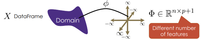
- use \(\phi\) to transform features
Feature Functions Examples
- Constant Feature Function: adding another vector as
bias term 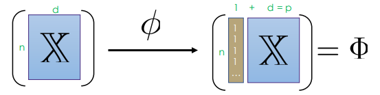
- aka constant feature, offset, intercept term, bias
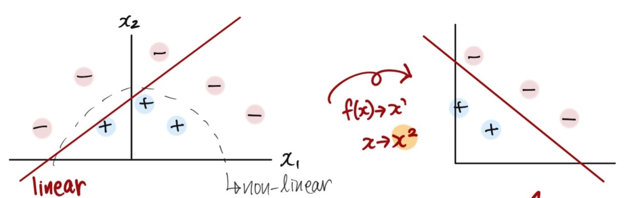
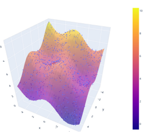
- Modeling Non-linear Relationships
-
apply non-linear function (like \(sin()\)) \(\Rightarrow\) may be easier to optimize
- \[f_{\theta}(x) = \theta _0 + \theta _1 x_1 + \theta _2 x_2 + \theta _3sin(x_1+x_2)\]
-
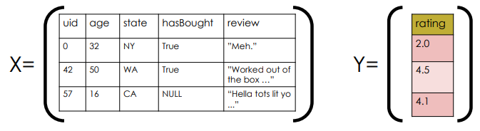
- cannot use \(X\) and \(Y\) in linear model because of text, categorical data, missing values …etc
Basic Transformations
- Uninformative Features:
like `UID` - \(transformation\): Remove
- Quantitative Features
like `Age` - \(transformation\): may apply non-linear transformations
like Log - \(transformation\): Normalize/Standardize
like (x-mean)/stdev
- \(transformation\): may apply non-linear transformations
- Categorical Features
like `State` - simply assiging values
(Alalbama=1, .., Utah=30) may indicate that those values have meaning (order / magnitude) NOT PREFERABLE - \(transformation\): One-hot-Encode
- simply assiging values
- Missing Values
- Quantitative:
- estimate and fill in (tricky)
like substituting mean - add another feature (boolean) named
missing_col_name- sometimes missing data can be a signal
- Categorical: (2) above (add additional category)
One hot Encoding (Dummy Encoding) 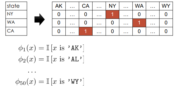
Bag of Words Encoding 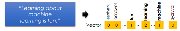
- bag: multiset (unordered collection which may contain multiple instance of each element)
- stopwords typically removed
- problems:
- too long and inefficient (high dimension but sparse)
- word order information lost (no context) \(\Longrightarrow\)
N-gram - new unseen words dropped \(\Longrightarrow\) add
unkown_columnfor counting unseen words
N-Gram Encoding
- when word order matters
- problem: further inefficiency problem
Wrap up
- feature transformations to capture domain knowledge
- introduces additional infromation
- bag of words can be used in autocompletion
- Feature Engineering Problems
- redundant features
- too many features
- overfitting