10 Optimization
in Notes / Dataanalytics / Datascience
Introduction
-
training most difficult optimization task
- very important but very expensive (특수기술 필요)
- examples:
- training -
learning optimal parameters (weights/biases) from data - model selection -
tuning hyperparameters (ex: learning rate)
- training -
- widely used:
- Stochastic Gradient Descent (SGD) and its variants
- Second-order methods
- often too expensive to compute/store Hessian \(\Rightarrow\) memory-efficient tech emerging
- Convex Optimization (블록최적화): 중요하지만 DL에서 거의 쓸모X
- Derivatives and Optimizaion Order
- derivatives
- First Derivative (=gradient) \(\Rightarrow\)
slope (Jacobian) - Second Derivate \(\Rightarrow\)
curvature (Hessian)
- First Derivative (=gradient) \(\Rightarrow\)
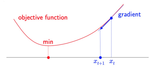
- optimization
- First-order algorithms : use only gradient
- \(x_{t+1}=x_t - \epsilon f'(x_t)\)
- \(x_{t+1}=x_t - \epsilon f'(x_t)\)
- Second-order algorithms : also use Hessian matrix (aka Newton’s method)
- \(x_{t+1}=x_t - \frac{f'(x_t)}{f''(x_t)}\)
- \(x_{t+1}=x_t - \frac{f'(x_t)}{f''(x_t)}\)
- First-order algorithms : use only gradient
- derivatives
- Critical Points (stationary points)
- points with zero slope: \(\nabla _x f(x) = 0\)
- Derivative gives no info about which direction to move
- Three types: maxima, minima, saddle point
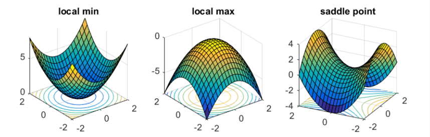
-
saddle point : both positive & negative curvature exist
- \(f(x)\) \(=x_1^2-x_2^2\)
- along \(x_1\) axis: \(f\) curves upward (local minimum)
- along \(x_2\) axis: \(f\) curves downward (local maximum)
- use of second derivative:
- characterize critical points
- measure curvature
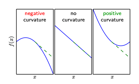
- (i) negative curvature: \(f\) decreases faster than gradient predicts
- (ii) no curvature: predicted correctly
- (iii) positive curvature: \(f\) decreases slower than predicted \(\Rightarrow\) eventually increases
- predict performance of an update in gradient based opt.
- In Deep Learning:
- in high dimension: saddle points more common than local minima
- obj function : many local minima + saddle points inside flat region \(\longrightarrow\) optimization difficult
- \(\Rightarrow\)
find a very low value of f (not necessarily minimal)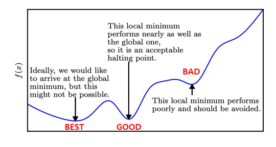
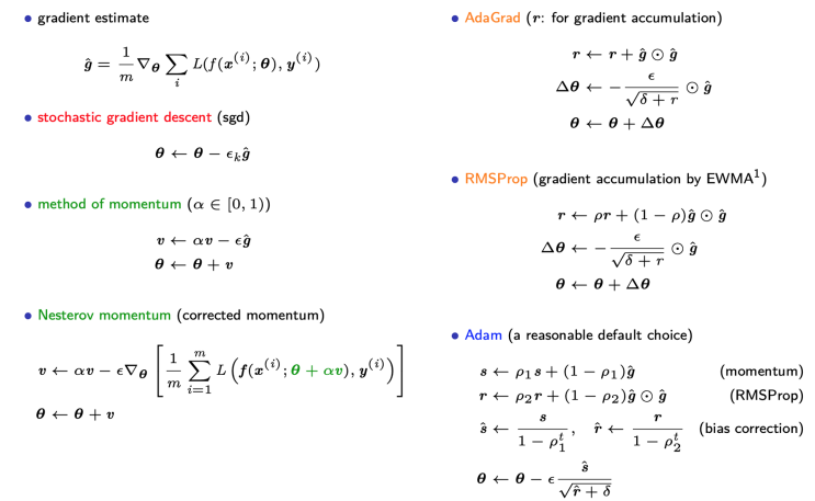
Gradient-based Optimization
Gradient Descent and its Limitations
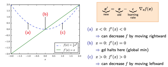
- derivative: useful for minimizing a function
- reduce \(f(x)\) by moving \(x\) in small steps with opposite sign of derivate
- can obtain unbiased estimate of gradient ???
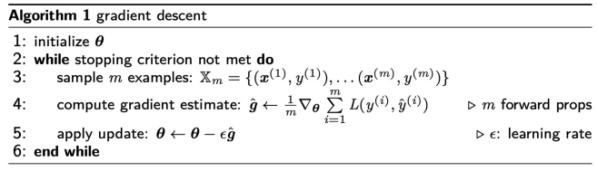
- sgd and its variants (\(N\): total # of examples)
- \(m=1\): sgd
- \(1<m<N\) : mini-batch sgd (typical \(m\): 64, 128, 256, 512)
- \(m=N\): batch gradient descent
Properties of SGD
- GOOD:
- number of training examples does not affect computation time per update
- most important, allows convergence even with big # of examples
- SGD works better in practice than theory
- number of training examples does not affect computation time per update
- BAD:
- Local minima and Saddle points
- Zero Gradient (Gradient descent gets stuck)
- Gradient Noise
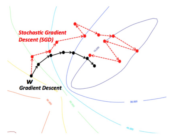
- Poor conditioning of \(H\)
- Poor Conditioning of H
- point \(x\) in multiple dimensions \(\rightarrow\) different second derivate for each direction
-
Condition Number of Hessian at \(x\) :
how much second derivatives differ from each other
- condition number of matrix with eigenvalues \({\lambda}\) : \(max_{i,j}\mid \frac{\lambda _i}{\lambda _j} \mid\)
if\(H\) have large condition # (poorly conditioned):- Gradient Descent Performs poorly
- 한쪽방향: deriv. increases rapdidly, 다른쪽: increase slowly
- GD unaware of this change in the derivative
- Difficult to choose \(\epsilon\)
- Gradient Descent Performs poorly
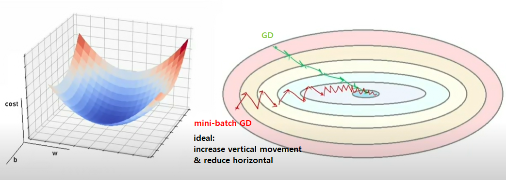
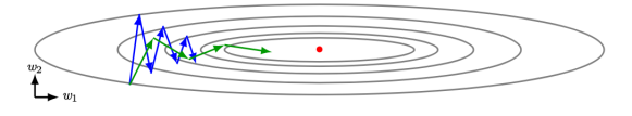
- Example: Assume Hessian \(H\)’s condition number =
5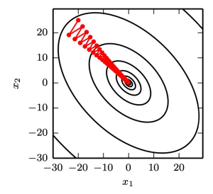
- most curvature: 5 times more curvature than least (long canyon)
- most curvature: direction \([1,1]\nearrow\)
- least curvature: direction \([1,-1]\searrow\)
- Gradient Descent (red lines): slow (zig-zag)
- methods considering \(H\) : can predict: steepest direction not promising
- \(\Rightarrow\) how to handle poor conditioning without directly considering \(H\)?
Exponentially Weighted Average (EWMA)
Given: time series \(g_1, g_2, \cdots\), EWMA : \(v_t = \begin{cases} g_1 & t=1 \\ \alpha v_{t-1}+(1-\alpha)g_t & t> 1\end{cases}\)
- \(v_t\): EMWA at time \(t\)
- \(g_t\): observation at time \(t\)
- \(\alpha \in [0,1]\): degree of weighting decrease (constant smoothing factor, 주로
0.9) - Example: gas price over time
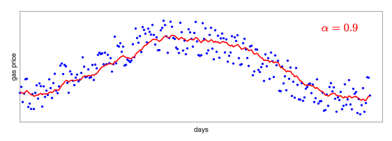
- \(v_t\) \(= \alpha \cdot\) \(v_{t-1}\) \(+(1-\alpha) \cdot\) \(g_t\)
- blue dots: gas price g
- red curve: EWMA v
- Effective weighting decreases exponentially over time:
- \(v_t\) \(=\alpha v_{t-1}+(1-\alpha)g_t\)
- = \(\alpha[\alpha v_{t-2}+(1-\alpha)g_{t-1}] +(1-\alpha)g_t\)
- \(=\) …
\(=\alpha ^k v_{t-k}+(1-\alpha)\) \([g_t + \alpha g_{t-1}+\alpha ^2 g_{t-2}+\cdots+a^{k-1}g_{t-k+1}]\)
- \(\Rightarrow\) “exponentially weighted” (최근 데이터에 더 많은 가치를 두고 제일 옛날꺼에는 거의 안둠)
- Approximation:
- \(v_t\) \(=(1-\alpha)g_t + \alpha v_{t-1}\)
- \(=(1-\alpha)\) \([g_t + \alpha g_{t-1}+\alpha ^2g_{t-2} + \alpha ^3 g_{t-3} + \cdots]\)
- \(=\frac{g_t + \alpha g_{t-1}+\alpha ^2g_{t-2}+\cdots}{1+\alpha + \alpha ^2 + \cdots} \Rightarrow\) weighted average formula
- DENOMINATOR = effective number of observations:
- \(1+\alpha + \alpha ^2 + \cdots\) = \(\frac{1}{1-\alpha}\)
- bottom line : \(v_t \approx\) average over \(\frac{1}{1-\alpha}\) last time points
- ex) \(a=0.9\) : average over 1/(1-0.9) = 10 points
- Effect of Smoothing Factor
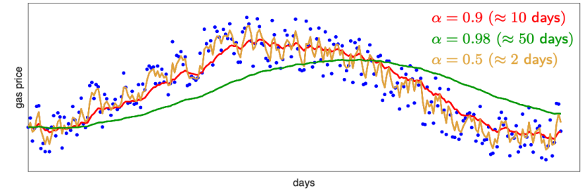
- Higher \(\alpha \Rightarrow\) more weight to past, less weight to present
- Smoother Curve \(\leftarrow\) averaging over more days
- Shifted further \(\leftarrow\) averaging over larger window
- Curve adapts more slowly to changes with more latency
- Higher \(\alpha \Rightarrow\) more weight to past, less weight to present
- Bias Correction
- 첫 몇개의 샘플은 충분한 데이터가 안 쌓였기 때문에 inaccurate average
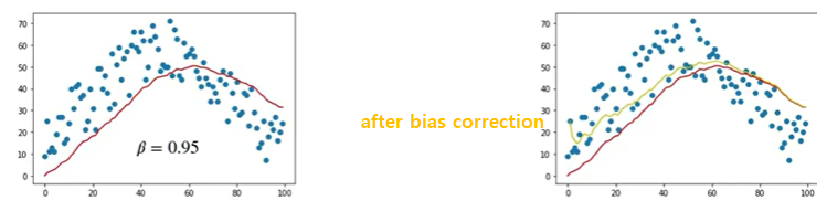
- instead of \(v_t\), use \(\frac{v_t}{1-\alpha ^t}\)
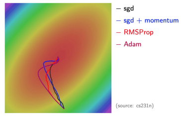
Gradient Descent with Momentum
- sgd: popular but sometimes slow
- method of momentum (Polyak, 1664):
- designed to accelerate learning, even though
- high curvature
- small but consistent gradients
- noisy gradients
- can be combined to existing sgd variants
- designed to accelerate learning, even though
- Common Algorithm: accumulates exponentially decaying moving average of past gradients \(\rightarrow\) continue to move in that direction
Momentum applied to three forms of SGD
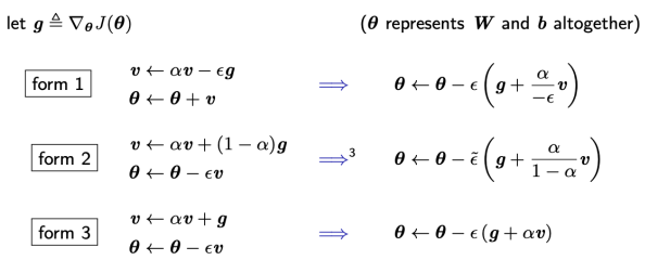
- \(\theta\) updated by linear combination of gradient and velocity
- \(\theta \leftarrow \theta - \epsilon(\) \(g\)\(+ constant \cdot\) v \()\)
Nesterov Momentum
- difference :
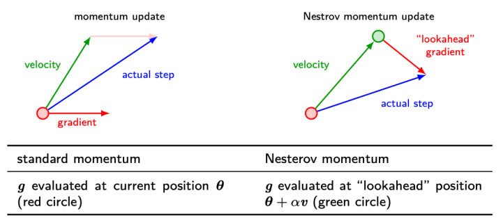
- standard: gradient \(g = \nabla _\theta J\) evaluated at current position \(\theta\) (red circle)
- Nestrov: \(g\) evaluated at lookahed position \(\theta + \alpha v\) (green circle), after current velocity is applied
- \(\Rightarrow\) add
correction factor - \[v \leftarrow \alpha v - \epsilon \nabla _\theta J(\theta + \alpha v)\]
- \[\theta \leftarrow \theta + v\]
- \(\Rightarrow\) add
- Advantages:
- Stronger theoretical converge guarantees for convex functions
- Standard Momentum보다 나음
Per-parameter Adaptive learning Rates
- adaptively turn \(\epsilon\) for each parameter
- goal: move horizontally BUT huge vertical oscillations
- \(\Rightarrow\) Solution: slow down learning vertically, speed up (적어도 유지) horizontally
- 실제 구현 방법 (without relying on \(H\))
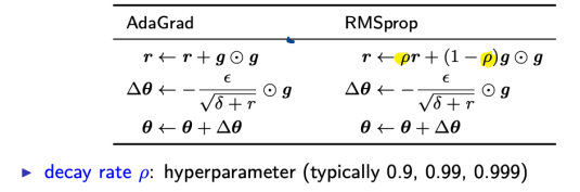
1. AdaGrad
- individually adapts learning rate of each direction (each parameter)
- steep direction: slow down learning
- gently sloped direction: speed up learing
- adjusts learning rates per parameter:
- \(\epsilon _j =\) \(\frac{\epsilon}{\sqrt{\sum_{all \hspace{0.1cm}previous \hspace{0.1cm}iterations}(g_j \cdot g_j)}}\)
- \(\epsilon\): global learning rate
- \(\epsilon _j\): learning rate of dimension \(j\) (parameter \(\theta _j\) )
- \(g_j = \frac{\partial J(\theta)}{\partial \theta _j}\) : gradient wrt dimension \(j\)
- GOOD: greater progress in more gently sloped directions
- BAD (esp in DL): monotonically decreasing \(\epsilon\): too aggressive + stops learning too early
- Adadelta: extension of Adagrad
- restricts accumulated past gradients
- reduces aggressive \(\epsilon\)
2. RMSProp
root-mean-squaure prop
- modified AdaGrad (non-convex setting에서도 잘 돌아가게)
- Change gradient accumulation to EWMA
- exponentially decaying average (\(\rho\)) 사용
- 아주 오래된 history 삭제
- converge rapidly after finding convex bowl
3. Adam
adaptive moment estimation (RMSProp + momentum + bias correction)
- for each iteration:
- compute gradient \(g\)
- update first moment: \(s \leftarrow \rho _1 s+(1- \rho _1) g \hspace{2cm} \leftarrow\) “momentum”
- update second moment: \(r \leftarrow \rho _2 s+(1- \rho _2) g \bigodot g\hspace{2cm} \leftarrow\) “RMSProp”
- bias correction: \(\hat{s} \leftarrow \frac{s}{1-\rho _1 ^t}, \hspace{2cm} \hat{r} \leftarrow \frac{r}{1-\rho _2 ^t}\)
- update parameter: \(\theta \leftarrow \theta - \epsilon \frac{\hat{s}}{\sqrt{\hat{r}+\sigma}}\)
Full algorithm
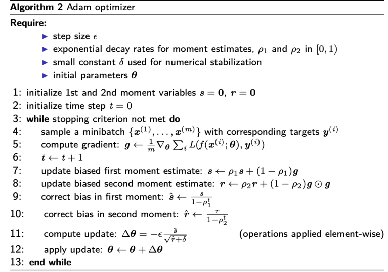
- often works better than RMSProp, recommened as default
- sgd + Nestrov Momentum도 해볼만 함
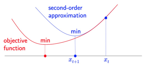
Second-order Optimization
Idea behind Newton’s Method
- considering Taylor Series approximation: \(f(x) \approx f(x^{(0)})+(x-x^{(0)})^Tg + \frac{1}{2}(x-x^{(0)})^TH(x-x^{(0)})\)
- gradient: \(f'(x)\)
- Hessian: \(f''(x)\)
- at point \(x_0\):
- \(f(x) \approx f(x_0) + (\) \(x\) \(-x_0)f'(x_0) + \frac{1}{2}(\) \(x\) \(-x_0)^2f''(x_0)\)
- \(f'(x)\) \(=f'(x_0)+(x-x_0)f''(x_0)\)
respect to x - \(0 = f'(x_0) + (x-x_0) f''(x_0)\)
set to zero - \(0 = f'(x_0) + xf''(x_0) - x_0f''(x_0)\)
solve for x - \(xf''(x_0) =\) \(x_0f''(x_0)-f'(x_0)\)
- \[x= x_0 - \frac{f'(x_0)}{f''(x_0)}, \hspace{1cm} \longrightarrow x_0 - \frac{g}{H}\]
Newton’s Update Rule : \(x^* = x^{(0)}-\) \(H^{-1}\)\(g\)
- PROS: No hyperparameter (in theory)
- gradient requires \(\epsilon\) (hyperparameter) but this doesn’t
- CONS: Inefficiency (\(H : O(n^2)\) elements, \(H^{-1}\) takes \(O(n^3)\) for inverting) \(\Rightarrow\) 안쓰는 이유
- PROS: No hyperparameter (in theory)
- IDEA:
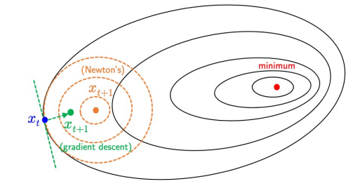
- get second-order approximation and minimize \(\Rightarrow\) faster than GD
Quasi-Newton Methods
- avoid directly inverting \(H\) \(\rightarrow\) reduce comparison time (\(O(n^3) \rightarrow O(n^2)\))
- approximate \(H^{-1}\) with Matrix \(M_t\)
- \(M_t\): iteratively refined by low-rank updates
- determine direction of descent by \(\rho _t = M_tg_t\) and update: \(\theta _{t+1} = \theta _t - \epsilon \rho _t\)
- BFGS algorithm (Broyden-Fletcher-Goldfarb-Shanno)
- most popular quasi-Newton method
- still requires \(O(n^2)\) memory to store \(H^{-1}\)
- L-GFGS (limited memory BFGS): doesn’t form / store full \(H\)
- full batch / deterministic mode: usually GOOD
- minibatch / stochastic setting : BAD
Summary