08 Linear Regression

18 Apr 2023 in Notes / Dataanalytics / Datascience

• Introduction
  • Regression
  • Linear Regression
• Linear Regression Algorithm
  • Matrix Representation
  • Minimization
  • Comments
• Interpretation via Hat Matrix

Introduction

• linear model:
  • set of lines
  • good first choice because
    • 1) Small VC (Vapnik-Chervonenkis) dimensions
    • 2) Generalize well (even with test data)
• Three Important Problems in Machine Learning
  1. Classification \(\rightarrow\) PLA
  2. Regression

     \(\rightarrow\) this chapter

  3. Logistic Regression (Probability Estimation) \(\rightarrow\) beginning of Deep Learning

Regression

• statistcal method to study relationship between \(x\) and \(y\):
  • \(x\): aka covariate / predictor variable / independent variable / feature
  • \(y\): aka response / dependent variable / Ground Truth
• Training Data \((x_1, y_1), ..., (x_N, y_N)\)
  • assume that noise is in our data (\(\rightarrow\) learning more practical )
  • Noise \(\epsilon\) added to target: \(y_n = f(x_n) + \epsilon\)
  • \(y \tilda P(y\mid x)\) instead of \(y=f(x)\)
• GOAL: find model \(g(x)\) that approximates \(y_n\)

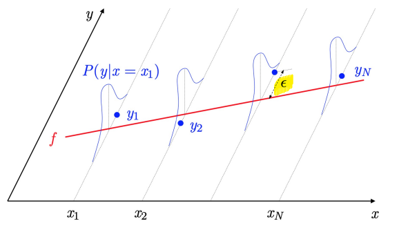
• \(y_i\) = \(f(x_i) + \epsilon\)

• assumption: homoscedasticity (each variance are same)

• \(re\) (back) + \(gression\) (going) = going back from data to formul - Sir Francis Galton
  • regression towards the mean

Linear Regression

• popular linear model for predicting quantitative response
  • applies to real-valued target functions
• Types of Linear Regression
  • simple linear regression ( \(d=1\) ) : one predictor \(\leftarrow\) learn this right now
  • multiple linear regression: ( \(d>=2\) ) : multiple predictor
• how to solve linear regression problem:
  1. Least Squares
     • (OLS) Ordinary Least Squares
     • Generalized Least Squares: homoscedasticity X
     • Iteratively Reweighted Least Sqaures: no need for invert matrix
  2. Maximum Likelihood: Ridge/Lasso, Least Absolute…etc
  3. Others : Bayesian, Principle…etc
• Example: Credit Approval Revisited
  • regression problem (rather than classification) (ex: set credit limit for each customer)
  • bank uses historical records to build dataset \(\mathbb{D}\)
    • \(\mathbb{D}\): \((x_1,y_1), ..., (x_N, y_N)\)
    • \(x_n\): customer information
    • \(y_n\): credit limit (set by human experts) \(\leftarrow\) real number
  • \(g\): what we are looking for (how human experts determine credit limits)
    • target: not deterministic function \(y=f(x)\), but \(NOISY\) Target (there is more than one human expert)
      • formalized as a distribution of a random variable
  • \(y_n\) (Regression Label) from \(P(y\mid x)\) instead of \(f(x)\)

Linear Regression Algorithm

\[E_{out}(h) = \mathbb{E}[(h(x)-y)^2]\]

• minimizing (expected value of error) squared error between \(h(x)\) and \(y\)
• using MSE (\(w^Tx-y\))
• GOAL: find \(h\) that achieves a small \(E_{out}(h)\)
• Issue: \(E_{out}\) cannot be computed (\(P(x,y)\) is unknown)
• \(\Rightarrow\) turn to in-sample error

\(E_{in}(h) = \frac{1}{N}\sum_{n=1}^N(h(x_n)-y_n)^2\)

• instead of using estimated error, use average of error
• In linear regression, \(h\) takes form of linear combinations of components of \(x\):
  • \[h(x) = \sum_{i=0}^dw_ix_i = (w^Tx)\]
  • \((w^Tx)\) aka signal
  • \(\rightarrow\) in-sample error can be re-written:
    • \(E_{in}(h)\)=\(\frac{1}{N}\sum_{n=1}^N(w^Tx-y_n)^2\)
    • find optimal w
• Linear Model Conditions
  1. \(E_{in}\) \(\approx E_{out}\)
  2. \(E_{in}\) is small enough

Matrix Representation

\(X=\begin{bmatrix} 1, x_1\\1, x_2\\1, x_3\\1, x_4\end{bmatrix}, w = \begin{bmatrix}w_0\\w_1\end{bmatrix} y = \begin{bmatrix}y_1\\y_2\\y_3\\y_4\end{bmatrix}\)

• \(y = xw \Rightarrow\) linear model!
• in-sample error = function of \(w\) and data \(X, y\):
  • (1) \(E_{in}(w) = \frac{1}{N}\sum_{n=1}^N(w^Tx-y_n)^2\)
  • (2) \(=\frac{1}{N} \left\lVert\begin{bmatrix}x_2^Tw-y_2\\x_1^Tw-y_1\\...\\ x_n^Tw-y_n\\\end{bmatrix} \right\rVert^2\)
    • \(\left\lVert \cdot \right\rVert\): Euclidean norm of vector
  • (3) \(= \frac{1}{N}\left\lVert xw-y \right\rVert^2\)
    • = \(\frac{1}{N}((xw-y)^T(xw-y))\)
    • = \(\frac{1}{N}((w^Tx^T - y^T)(xw-y))\)
    • = \(\frac{1}{N}(w^Tx^Txw - w^Tx^Ty - y^Txw + y^y)\)
  • (4) \(\frac{1}{N}(w^Tx^Txw - 2w^Tx^Ty + y^y)\)
    • tip (\(y^TXw = (w^TX^Ty)^T = w^TX^Ty\))
      Example

      \[X=\begin{bmatrix} 1, x_1\\1, x_2\\1, x_3\\1, x_4\end{bmatrix}, w = \begin{bmatrix}w_0\\w_1\end{bmatrix} y = \begin{bmatrix}y_1\\y_2\\y_3\\y_4\end{bmatrix}\]

      • \[E_in(w)=\frac{1}{4} \sum_{i=1}^4(w^Tx_n-y_n)^2\]
      • = \(\frac{1}{4} \left\lVert \begin{bmatrix} 1, x_1\\1, x_2\\1, x_3\\1, x_4\end{bmatrix} \begin{bmatrix}w_0\\w_1\end{bmatrix} - \begin{bmatrix}y_1\\y_2\\y_3\\y_4\end{bmatrix} \right\rVert^2\)
  • (5) \(w_{lin} = argmin(E_{in}(w))\) (\(w_{lin}\) = solution)
  • (6) \(argmin \frac{1}{N} \left\lVert Xw-y \right\rVert^2\)

Minimization

• equation (4) implies \(E_{in}(w)\) is continous, differentiable, convex
  • \(\Rightarrow\) use standard matrix calculus to find \(w\) that minimizes \(E_{in}(w)\) by requiring \(▽E_{in}=0\)
  • other (gradient descent) also works

  

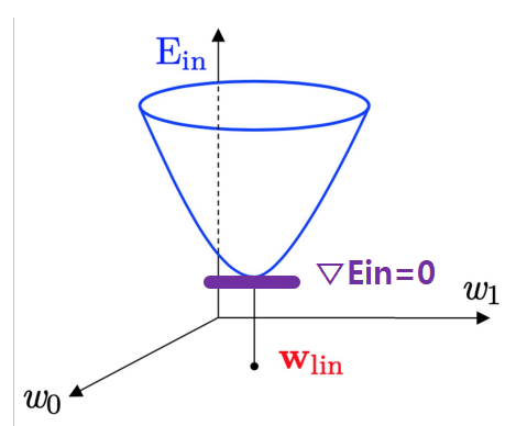
  • \(w_{lin}\): optimal value of \(w\)
• Recall:
  • Gradient identifies:
    • \(▽_w(w^TAw)\)=\((A+A^T)w\)
    • \(▽_w(w^Tb)\)=\(b\)
  • scalar \(w\)
    • \(E_{in}(w)\) = \(aw^2-2bw+c\)
    • \(\frac{∂}{∂w}E_{in}(w)\)= \(2aw-2b\)
  • vector \(w\)
    • \(E_{in}(w)\) = \(w^TAw-2w^Tb+c\)
    • \(▽E_{in}(w)\) = \((A+A^T)w - 2b\)
• Solution
  • from equation (4) \(\frac{1}{N}(w^Tx^Txw - 2w^Tx^Ty + y^y)\)
  • \(▽E_{in}(w)\) = \(\frac{2}{N}(X^TXw-X^Ty)\) set to 0
    • both \(w\) and \(▽E_{in}(w)\) = column vectors
  • solve for \(w\) that satisfies the normal equations
  • \(X^TXw\) = \(X^Ty\)
  • \(w =\) \((X^TX)^{-1}X^Ty\)
    • if \(X^TX\) is invertible, \(w=X^+y\) (mostly invertible)
      • (\(X^+\) (pseudo-inverse of X) = \((X^TX)^{-1}X^T\))
      • \(\Rightarrow w\) = unique optimal solution
    • else pseudo- inverse can still be defined but no unique solution
      • \(\Rightarrow\) multiple solutions for \(w\) that minimizes \(E_{in}\)
• Example
  Data

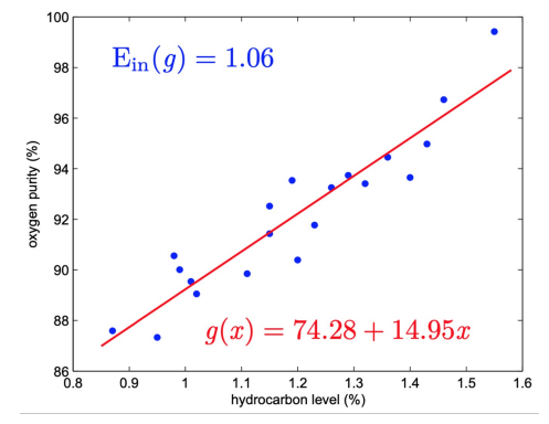
  • (20 rows each) data matrix \(X = \begin{bmatrix} 1, 0.99\\1,1.02\\1,1.15\\...\\1,0.95\end{bmatrix}\), target vector \(y= \begin{bmatrix}90.01\\89.05\\91.43\\...\\87.22 \end{bmatrix}\)
  • \(X^TX\) is invertible
    • \(X^TX\) = \(\begin{bmatrix}20.00, 23.92\\23.92,29.29 \end{bmatrix}\Rightarrow (X^TX)^{-1}=\begin{bmatrix}2.15,-1.76\\-1.76,1.47\end{bmatrix}\)
  • \((X^TX)X^Ty\) yields
    • \(w_{lin}\) = \(\begin{bmatrix}74.28\\14.95\end{bmatrix}\)
  • learned model:
    • \(g(x)\) = \(w_{lin}^Tx\) = \(74.28+14.95x\)
  • error: (안배움)
    • \(E_{in}(g)\) = \(1.06\)
    • \(E_{out}(g)\) \(\approx 1.45\)

  

Comments

• linear regression algorithm (aka OLS (ordinary least squares))
• provides BLUE (Best Linear Unbiased Estimator)
• compared to PLA, doesn’t really look like learning
• hypothesis \(w_{lin}\) comes from analytic solution(matrix inversion/multiplications) rather than iterative learning steps
• one-step learning \(\Rightarrow\) popular
• Linear Regression is a rare case
• there are methods for computing pseudo-inverse w/o interting a matrix

Interpretation via Hat Matrix

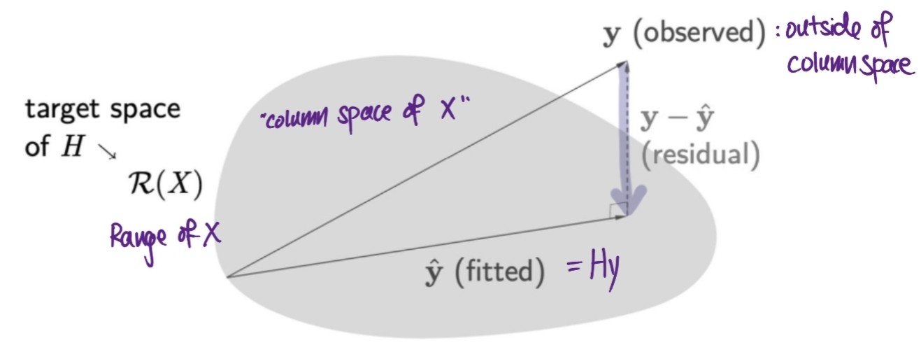
Hat Matrix (H)

(aka projection matrix)

• maps observed values (\(y\)) to fitted values(\(\hat{y}\))

• \[\hat{y} = Hy\]

• matrix \(H\) puts a hat on \(y\)

• Hat matrix in Linear Regression
  • linear regression weight vector \(w_{lin}\) attempts to map inputs \(X\) to outputs \(y\)
  • but does not produce \(y\) directly (only the estimate) due to ___ error
  • substitue expression for \(w_{lin}\) (assuming \(X^TX\) is invertible)
  • \(w_{lin}\) = \((X^TX)^{-1}X^Ty\)
  • and \(\hat{y}\) = \(Xw_{lin}\)
  • substitute \(\Rightarrow\)
  • \[\hat{y}= Xw_{lin} =X\cdot(X^TX)^{-1}X^Ty\]
  • \[\hat{y}= \Longrightarrow(X(X^TX)^{-1}X^T) \Longleftarrow y\]
  • \(\Rightarrow H = X(X^TX)^{-1}X^T\) : Hat matrix is actually a linear function

  \(\hat{y}\) : orthogonal projection of \(y\) on to the Range of X

  

• \(H\) is called projection/hat matrix iff \(H^2 = H\) (HHy=Hy, HHHHy=HY…)
• basic properties of hat matrix \(H\)
  1. symmetric: \(H^T=H\)
  2. idempotent: \(H^N=H\) (no effect on vectors already on space)
• for identy matrix \(I\):
  • \(I-H\) = also hat matrix
  • \((I-H)^2\) = \(I-2H+H^2\) = \(I-H\)
  • \(H^T(I-H) = 0 \Rightarrow\) target spaces are orthogonal
• trace
  • \(trace(H)\) = \(trace(X(X^TX)^{-1}X^T)\)
  • = \(trace(X^TX(X^TX)^{-1})\)
  • = \(trace(I)\)
  • = \(d+1\)

• for matrix \(A\), \(trace(A)\) = sum of diagonal \(\begin{bmatrix}O,-,-\\ -,O,-\\ -,-,O \end{bmatrix}\)

• since \(trace(H)\) = sum of diagonal elements in \(H\):
  • \(\Rightarrow\) \(trace(AB) = trace(BA)\)