Supervised Learning Linear Regression

27 Dec 2022 in Notes / Artificialintelligence / Introductiontoai

DAY 2

• Linear Regression
  • Linear Model
  • Cost Function
  • Cost Function Minimization (GDM)
  • Learning Rates α
• Multi-Variable Linear Regression
• Linear Regression Implementation
  • Python Libraries
  • PyTorch implementation of Linear Regression Model 🔥

Linear Regression

• 선형의 회귀분석
  

Linear Model

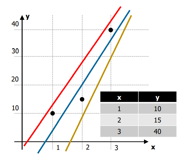
• graph analysis
  • blue line is the best model since it has the smallest error considering real data (points)
  • yellow line goes to negative in for the first point -> impossible

\[H(x) = Wx + b\]

• \(H\): Hypothesis
• \(W\): weight vectors
• \(b\): bias value

Cost Function

• aka Loss Function

\[Cost(W, b) = \frac {1}{m} \sum_{i=1}^m (H(x^i)-y^i)^2\]

• \(m\): number of training data (m빵)
  • the bigger the \(m\), the error rate (cost) will also become higher (데이터 많을수록 틀릴 가능성 high)
• \(H(x^i)\): expectation (예측치)
• \(y^i\): actual (실제값)
  • due to this \(y\) value, (actual data under linear model) the total value might become negative
  • ➡ square the whole expression (if set to \|absolute\|, then you can’t take the derivative of it)

Cost Function Minimization (GDM)

• \(W\)와 \(b\) needs to be found (\(x\) and \(y\) are constants)

• \(b\) ignored for convenience

• Grandient Descent Method
  

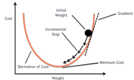
• \[W \leftarrow W - \alpha \frac {\partial} {\partial W} Cost(W)\]

1. find the slope of random point from Derivative of Cost
2. jump to point where slope is not as steep (jumping distance depends on steepness of a slope)
3. continue until \(W\) converges to 0

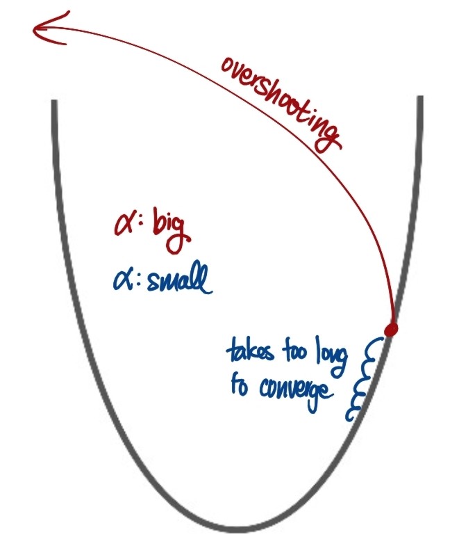
Learning Rates α

• \(\alpha\) : learning rate
• too large: overshooting

• too small: takes very long time to converge

  described in picture

  

• determining learning rates:
  • try several learning rates and observe the cost function

Multi-Variable Linear Regression

Model \[H(x_1,x_2, ..., x_n) = w_1x_1 + w_2x_2 + \cdots + w_nx_n + b\]

Cost \[Cost(W, b) = \frac {1}{m} \sum_{i=1}^m (H(x_i^i, x_2i, ..., x_n^i)-y^i)^2\]

• multiple \(x\) each require \(w\)
• more \(x\) leads to better accuracy (more information is provided)

Programming

• \[H(x_1,x_2, ..., x_n) = w_1x_1 + w_2x_2 + \cdots + w_nx_n + b\]
• ➡ \(H(X) = XW + b\)
• \[\begin{pmatrix} x_1 & x_2 & ... & x_n \end{pmatrix} \times \begin{pmatrix} w_1\\ w_2\\ ...\\ w_n \end{pmatrix} = w_1x_1 + w_2x_2 + \cdots + w_nx_n\]
• MATRIX MULTIPLICATION used for faster calculation (transpose \(W\))
• \[H(X) = XW_T + b\]

Linear Regression Implementation

Python Libraries

• in released order:

1. Tensorflow
   • by Google
2. PyTorch
   • my Meta
   • easier and more intuitive
3. Keras
   • by Google
   • only for deep nerual network architecture
   • easiest

PyTorch implementation of Linear Regression Model 🔥

import torch

# Training Data
x_train = torch.FloatTensor([[1,1], [2,2], [3,3]])
y_train = torch.FloatTensor([[10], [20], [30]])
                
                #dimensions of training data
W = torch.randn([2,1], requires_grad=True) #gradient descent Function
b = torch.randn([1], requires_grad = True) 
                            #mimmize (optimize parameters W, b)
optimizer = torch.optim.SGD([W, b], lr = 0.01) #Stochastic Gradient Descent 어쩌고...
                                    #learning rate (alpha) = 0.01
def model_LinearRegression(x):
  return torch.matmul(x, W) +b  #H(x) = Wx + b

for step in range(2000):  #LOOP! (jump 2000 times)
  prediction = model_LinearRegression(x_train)
  cost = torch.mean((prediction - y_train) ** 2)  #square값 해주고 m빵
  #알아서 optimizing 해줌
  optimizer.zero_grad() # 0까지 optimize
  cost.backward()       
  optimizer.step()

x_test = torch.FloatTensor([[4,4]]) #4,4 값 추가 시 예상 답: 40이 나와야 함
model_test = model_LinearRegression(x_test)
print(model_test.detach().item())

• larger loops (more tries) leads to better accuracy (closer to 40)