ANN Theory
DAY 5 - 6
- Introduction
- Multilayer Perception (MLP)
- PyTorch implementation for ANN (XOR)🔥
- Further ANNs
- Gradient Vanishing Problem
- Deep Learning Review
ANN: Aritificial Neural Network
Introduction
- Human Brain (Neuron) to Deep Learning Model via mathematical modeling (정보전달과정)
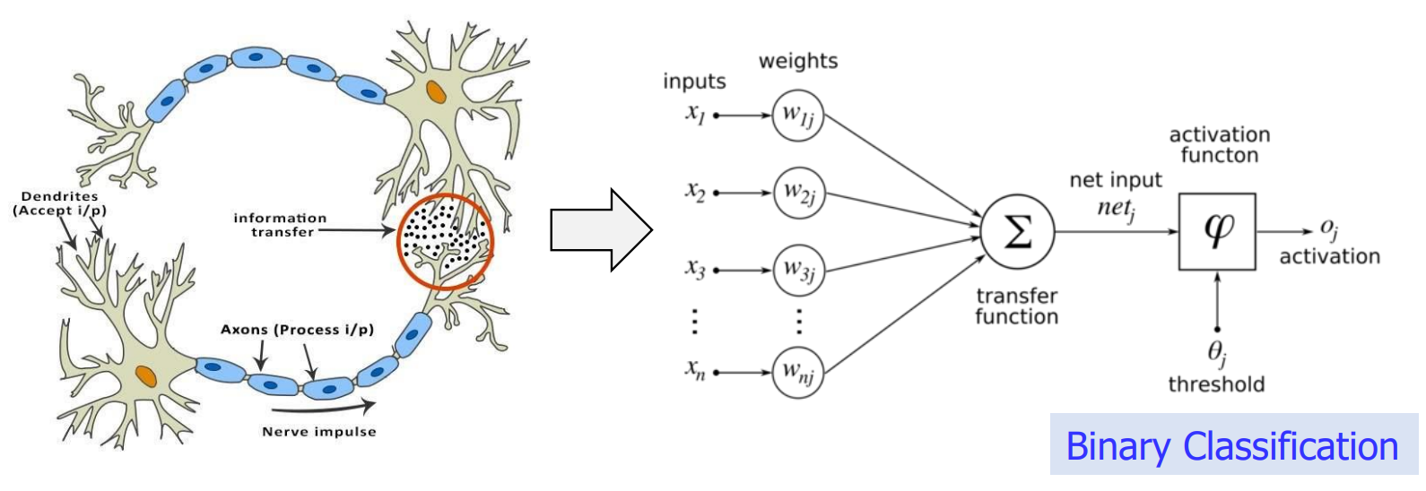
- inputs can be modified by weights
- amplification, decrease, or eliminated by *0
- result activated if passes threashold (BINARY CLASSIFICATION)
Multilayer Perception (MLP)
Proposed and Mathematically proven by Prof. Marvin Minsky at MIT (1969), “Father of AI” (who first made the term AI)
- NEURAL NETWORK ARCHITECTURE
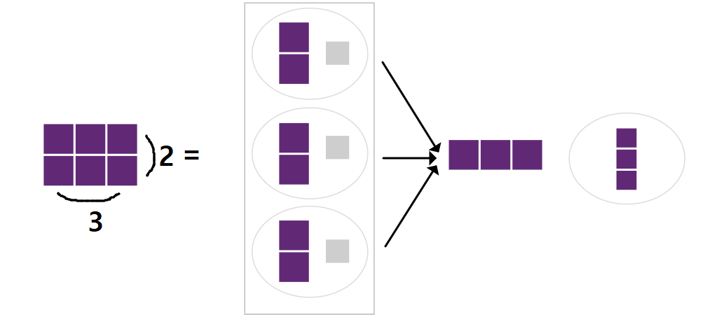
NN : Do Linear Classification a lot of times
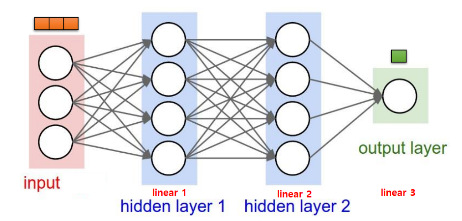
- 3-size inputs [x, y, z] => 1-size output
- 1 size output: linear regression or binary classification
- 2 or more: softmax classification
- Hidden Layers do additional Linear Classifications
- 3 Linear Classifications (indicating the model is nonlinear) => complex calculations are possible
Application to Logic Gate Design
- AND, OR Gates
- Binary Classification is possible)
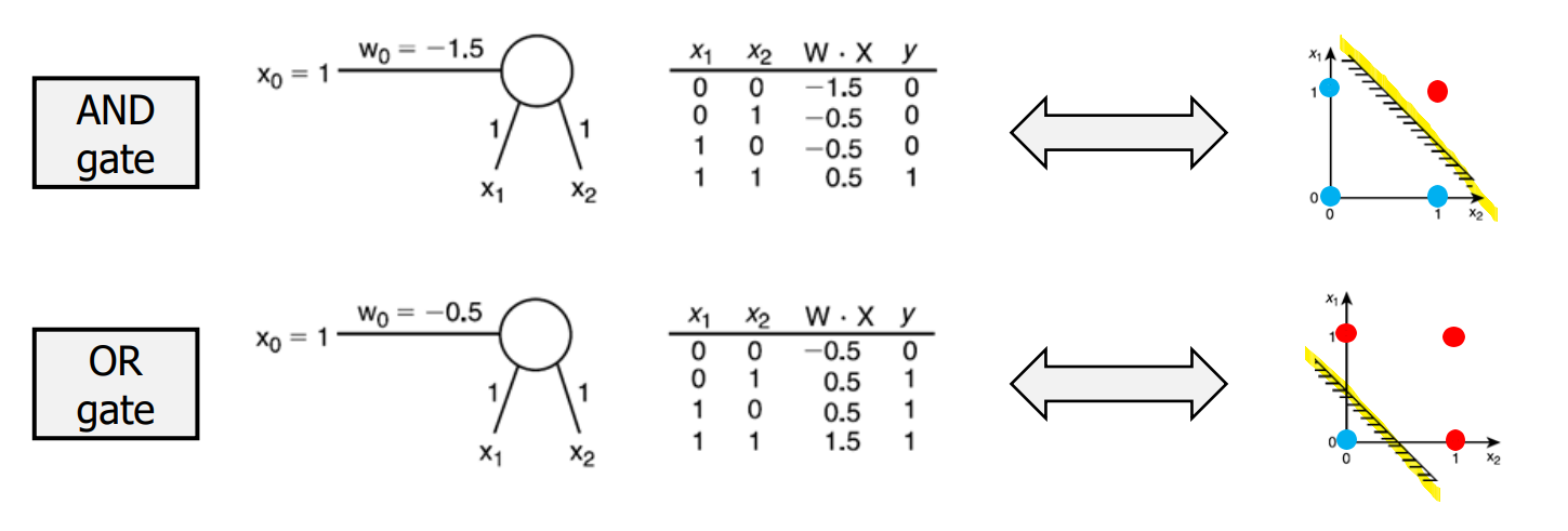
- points can be divided into 2 parts depending on y [0, 1]. (red, blue)
- XOR Gate
XOR Gate = Same ? 0 : 1
- why hidden layer was first created
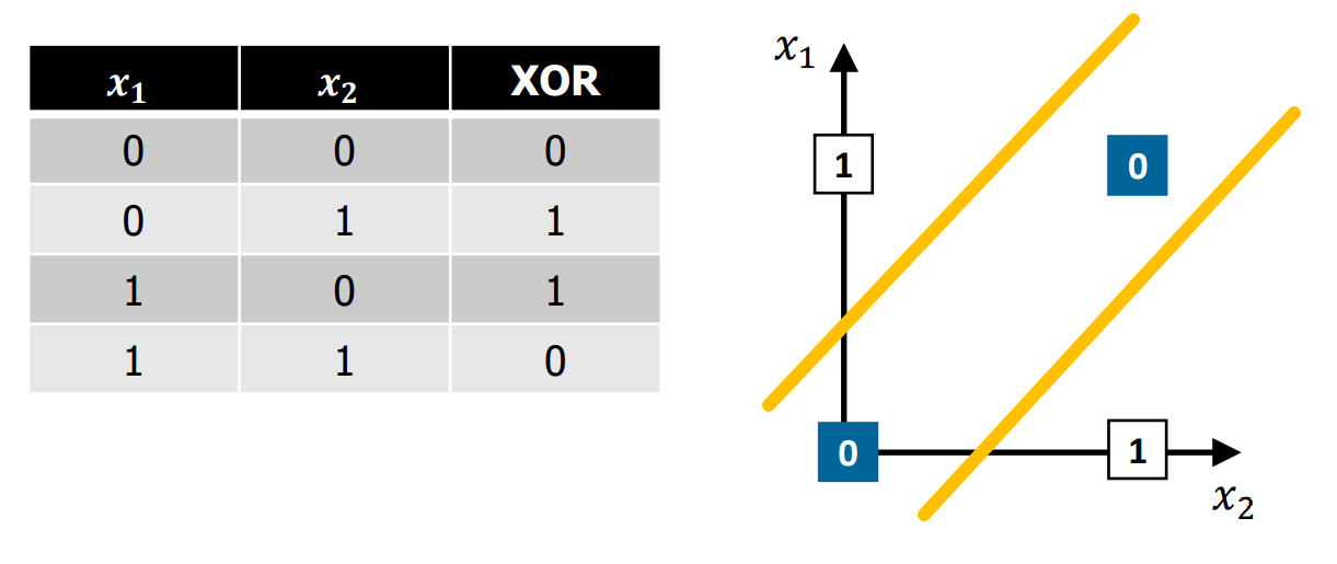
requires 2 linear classification
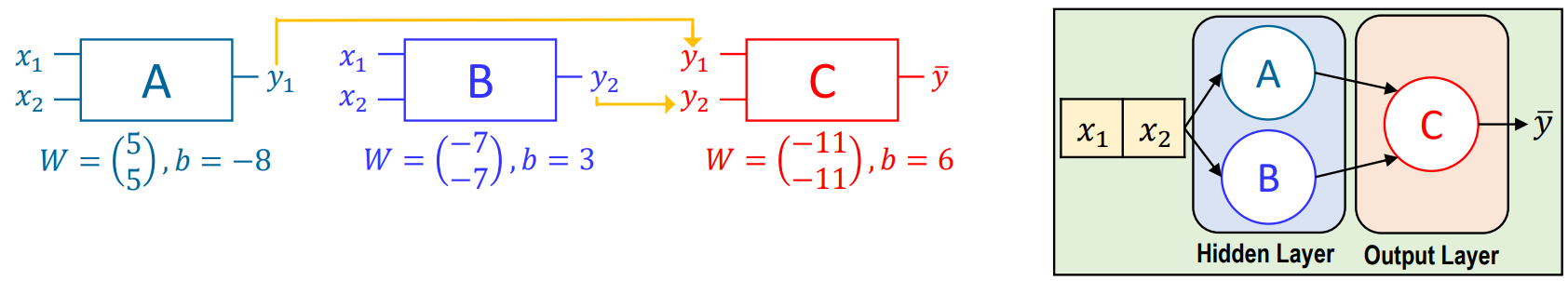
Solving XOR with MLP
- \(\bar y\) = XOR
| \(x_1\) | \(x_2\) | \(y_1\) | \(y_2\) | \(\bar y\) | XOR |
|---|---|---|---|---|---|
| 0 | 0 | 0 | 1 | 0 | 0 |
| 0 | 1 | 0 | 0 | 1 | 1 |
| 1 | 0 | 0 | 0 | 1 | 1 |
| 1 | 1 | 1 | 0 | 0 | 0 |
- proves that hidden layers allow unsolvable problems solvable
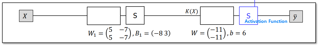
Forward Propogation
can we add another hidden layer?
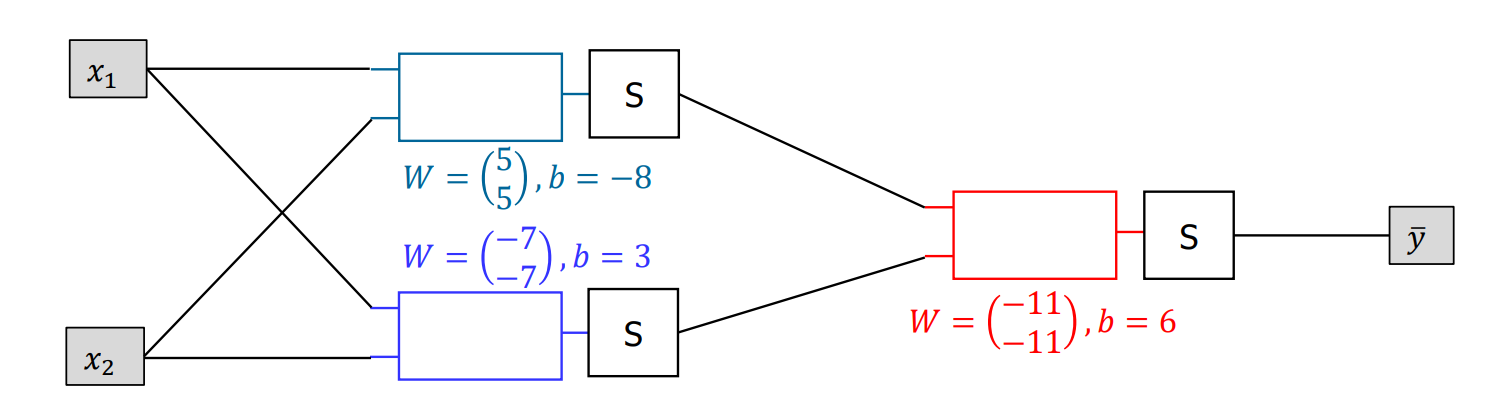
Then new W \(\begin{pmatrix} ? \\ ? \end{pmatrix}\) and \(b\) required for new \(S\) and \(W=\begin{pmatrix} -11 \\ -11 \end{pmatrix}\) (red box) ➩ \(W = \begin{pmatrix} -11 \\ -11 \\ ? \end{pmatrix}\)
Toy Model
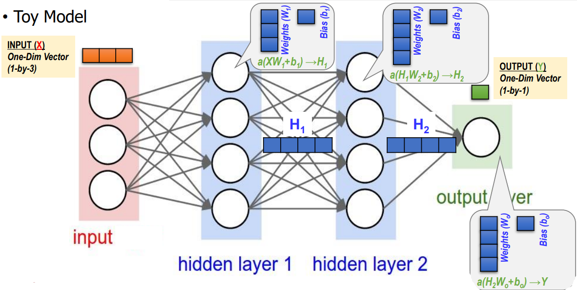
- although hidden layer 1 and hidden layer 2 looks alike, their weight vectors have the different size (different size inputs)
PyTorch implementation for ANN (XOR)🔥
import torch
import numpy as np

# Training Data
x_train = torch.FloatTensor([[0, 0], [0, 1], [1, 0], [1, 1]]) #XOR DATA
y_train = torch.FloatTensor([[0], [1], [1], [0]])

nHL = 3

W_h = torch.randn([2, nHL], requires_grad=True) # hidden layer weight
b_h = torch.randn([nHL], requires_grad = True)
W_o = torch.randn([nHL, 1], requires_grad=True) # ouput layer weight
b_o = torch.randn([1], requires_grad=True)

optimizer = torch.optim.SGD([W_h, W_o, b_h, b_o], lr = 0.01)

def model_ANN(x):
  HL1 = torch.sigmoid(torch.matmul(x, W_h) + b_h) #hidden layer with 3 units (먼저 생성)
  Out = torch.sigmoid(torch.matmul(HL1, W_o) + b_o)
  return Out

for step in range(200000):
  prediction = model_ANN(x_train)
  cost = torch.mean( (-1) * ((y_train*torch.log(prediction) + (1-y_train)*torch.log(1-prediction))))
  optimizer.zero_grad() # 0까지 optimize
  cost.backward()
  optimizer.step()

model_test = model_ANN(x_train)
print(model_test.detach().numpy())
Code Explanation
nHL = 3

W_h = torch.randn([2, nHL], requires_grad=True) # hidden layer weight
b_h = torch.randn([nHL], requires_grad = True)
def model_ANN(x):
  HL1 = torch.sigmoid(torch.matmul(x, W_h) + b_h) #hidden layer with 3 units (먼저 생성)
  Out = torch.sigmoid(torch.matmul(HL1, W_o) + b_o)
  return Out
input = [ [0, 0], [0, 1], [1, 0], [1, 1] ]
- Hidden Layer 추가 안할 시 output:
[ 0.5, 0.5, 0.5, 0.5]=> all are not> 0.5- =>
[ 0, 0, 0, 0 ] - ACTUAL: [ 0, 1, 1, 0 ] (50% accuracy) => HIDDEN LAYER REQUIRED
- =>
- Hidden Layer output :
[ 0.001413, 0.9953.., 0.993166..., 0.0079 ]=>[ 0, 1, 1, 0 ]=> CORRECT
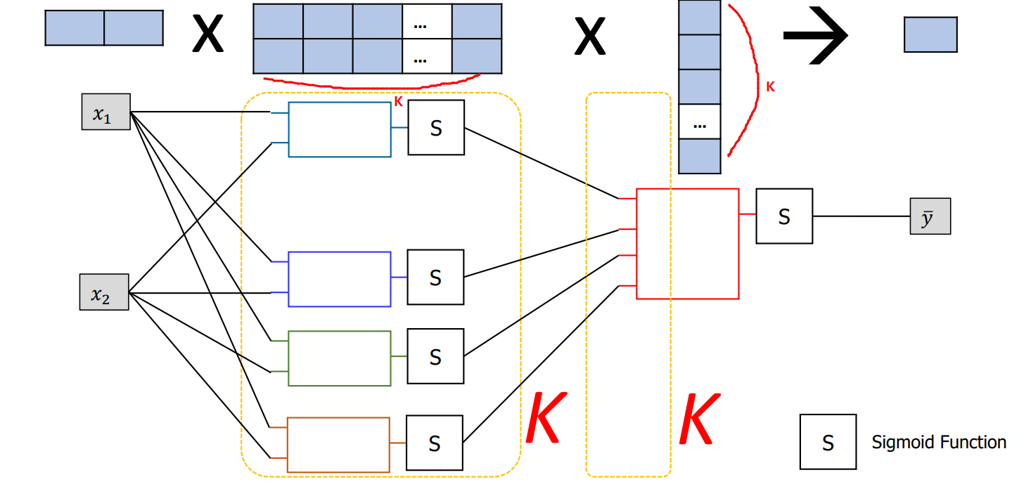
Further ANNs
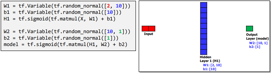
Wide ANN for XOR
(참고: tensorflow)
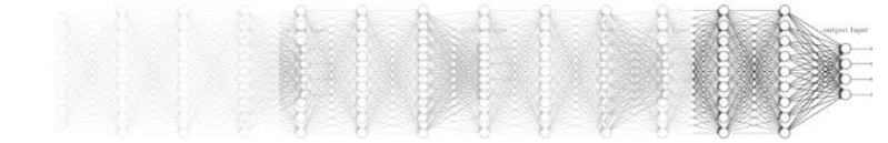
Deep ANN for XOR
(참고: tensorflow)
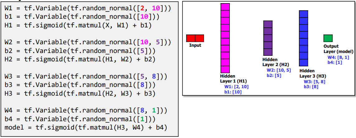
- More Layer the BETTER
Gradient Vanishing Problem
- No matter high the number of layers, accuracy can be low
- ex) 100000 as input -> mapped to 0 ~ 1 -> REPEAT -> … -> Value disappears (converges to 0)
RELU (Rectified Linear Unit)
- solves the Gradient Vanishing Problem
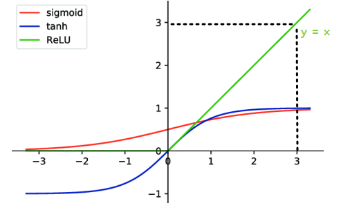
- when activated, the actual value is returned. ex) input 3, returns 3
Deep Learning Revolution
| 50 Years Ago | Now |
|---|---|
| labeled datasets too small | Big - Data |
| Computers too slow | GPU |
| only consider 1-D vector input | Conbolutional Layers for n-D inputs (Hidden Layers) |
| wrong type of non-linearity (activation function) | ReLU for Gradient Vanishing Problem |
Deep Learning Review
Deep Learning Computation Procedure
- Deep Learning Model Setup
- MLP, CNN, RNN, GAN, Costomized 중 뭐 쓸 것인지..
- Number of Hidden Layers, Units, Input/Outputs…
- Cost Function / Optimizer Selection
- Training (with Large-Scale Dataset)
- Input Data, Output: Labels
- Learning -> Weights Updates (\(W\) and \(b\)) for Cost Function Minimization
- Inference / Testing (Real-World Execution)
- Use \(W\) and \(b\) (optimized at step #2) to calculate input
- Input : Real-World Input Data
- Output: Inference Results based on Updated Weights in Deep NN