12 Decision Trees
in Notes / Dataanalytics / Datascience
- Introduction
- Decision Tree Basics
- Decision Tree Generation
- Restricting Decision Tree Complexity
- Random Forests
Introduction
- non-linear Classifiers
- non-linear decision boundary: add ‘non-linear’ features to linear model
ex: logistic reg - use non-linear learners
ex: nearest neighbors, decision trees, neural nets - K-Nearest Neighbor Classifier:
- simple, often a good baseline
- Can approximate arbitrary boundary: non-parametric
- Disadvantage: stores all data
- non-linear decision boundary: add ‘non-linear’ features to linear model
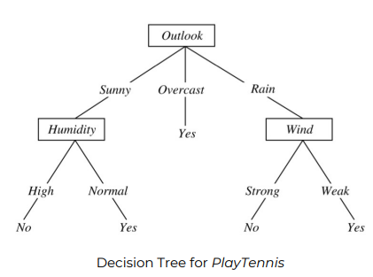
Decision Tree: a tree of questions that must be answered in sequence to yield predicted classification
- \(Y = (A\land B) \lor (\lnot A \land C)\) ((A and B) or (not A and C))
- one of the most intuitive classifer, easy to understand & construct
- 놀랍게도 굉장히 잘 된다
- Structure of Decision Tree
- internal nodes: attributes (features)
- Leafs: classification outcome
- Edges: assignment
- Example: Logistic Regression using petal data
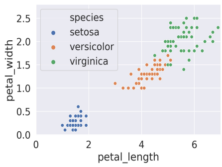
- logistic regression = linear \(\Rightarrow\) linear decision boundaries
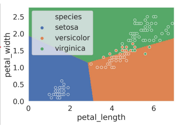
Decision Tree Basics
- seems good, gets every point correctly
- might result in overfitting
Decision Tree Generation
Traditional Algorithm
- all data starts in root node
- repeat until every node is either pure(one type) or unsplittable (duplicate but not splittable)
- pick best feature \(x\), best split value β
( x = petal_length, β = 2 ) - Split Data into 2 nodes ( x < β, x >= β )
- pick best feature \(x\), best split value β
- Learning Smallest (simplest) decision Tree :
NP-complete(existing algorithms exponential) - Use
Greedy Hueristics- start with empty tree \(\rightarrow\) choose next best attribute \(\rightarrow\) recurse \(\circlearrowleft\)
- Defining Best Feature
Node Entropy
\[node \hspace{0.1cm} entropy\hspace{0.1cm} S = -\sum _c p_c log_2p_c\]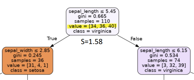
- Entropy of Root Node
- \(p_0=\) \(\frac{34}{110} = 0.31\)
- \(p_1=\) \(\frac{36}{110} = 0.33\)
- \(p_2=\) \(\frac{40}{110} = 0.36\)
- \(S =\) \(-(0.31 log_2(0.31)) -(0.33 log_2(0.33))-(0.36 log_2(0.36))\)
- \(S = 1.58\)
- Entropy = 혼란도: how unpredictable a node is
- LOW Entropy: more predictable \(\Rightarrow\) Good!
- HIGH Entropy: more unpredictble
- Entropy
- 0 Entropy: data all in one class (\(-1log_2(1)=0\))
- ex:
[ 34, 0, 0 ]\(\rightarrow p_0 = \frac{34}{34} = 1\) - \(-1 log_2 (1) =\) \(0\)
- ex:
- 1 Entropy: data evenly split between 2 classes
- ex:
[ 4, 4 ]\(\rightarrow p_0 = \frac{4}{8} = 0.5\), \(p_1 = \frac{4}{8} = 0.5\) - \(-0.5 log_2 (0.5) -0.5 log_2 (0.5) =\) \(1\)
- ex:
- 1.58 Entropy: split evenly into 3 classes
- ex:
[ 4, 4, 4 ]\(\rightarrow p_0 = p_1 = p_2 = \frac{4}{12} = 0.33\)- \(3 \times -0.33 log_2 (0.33) =\) \(1.58\)
- ex:
- \(\Rightarrow\) data evenly split between \(C\) classes
- \(C \cdot (\frac{1}{C}log_2(\frac{1}{C})) = -log_2(\frac{1}{C}) =\) \(log_2(C)\)
- 0 Entropy: data all in one class (\(-1log_2(1)=0\))
- Weighted Entropy as a Loss Function
- use it to decide which split to take
- given 2 nodes (\(X, Y\)) with each \(N_1, N_2\) samples:
- \[L=\frac{N_1S(X)+N_2S(Y)}{N_1+N_2}\]
- \(\Longrightarrow\) MIDTERM
- Defining Best Feature
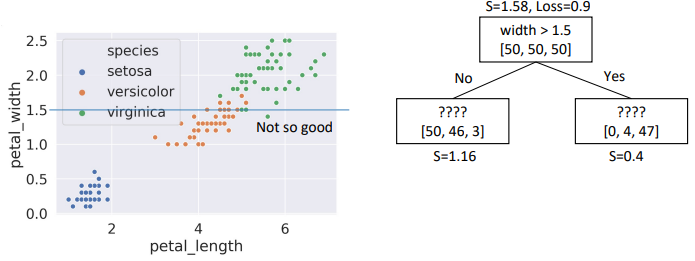
- Choice #1:
width > 1.5, child node entropies: \(entropy([50,46,2])=1.16\), \(entropy([4,47])=0.4\)- Weighted Average = \(\frac{99}{150}*1.16 + \frac{51}{150}*0.4 =\) \(0.9\)
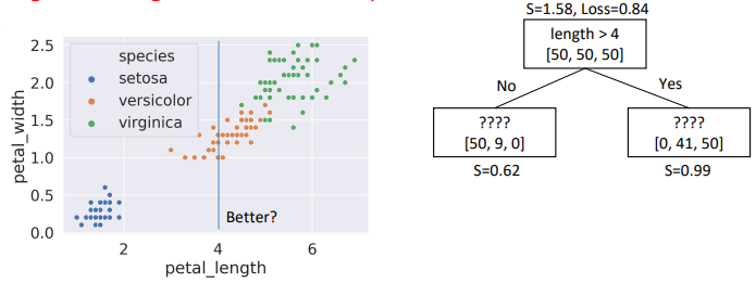
- Choice #2:
length > 4, child node entropies: \(entropy([50,9])=0.62\), \(entropy([41,50])=0.99\)- Weighted Average = \(0.84\) \(\Rightarrow\) Better than choice (1)
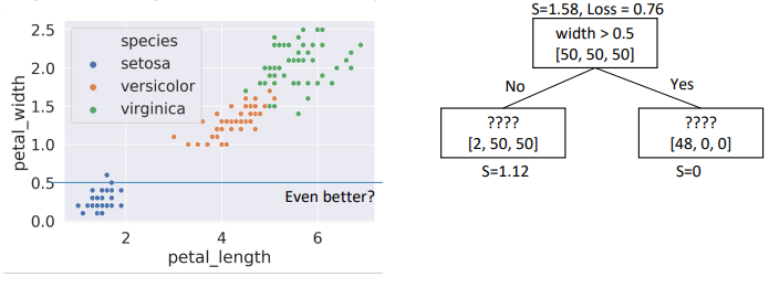
- Choice #3:
width > 0.5, child node entropies: \(entropy([2,50,50])=1.12\), \(entropy([48])=0\)- Weighted Average = \(0.76\) \(\Rightarrow\) Better than choice (2)
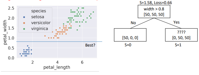
- Choice #4:
width > 0.9, child node entropies: \(entropy([50,50])=0.1\), \(entropy([50])=0\)- Weighted Average = \(0.66\) \(\Rightarrow\) Better than choice (3)
- Choice #1:
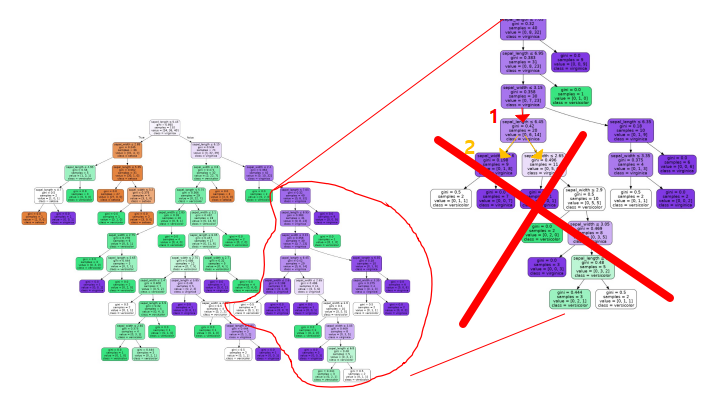
- \(\Rightarrow\) Traditional Decision Tree Generation Algorithm has overfitting issues
Restricting Decision Tree Complexity
- Approaches Explained
- Preventing Growth: set one or more special rules to prevent growth
- ex: don’t split nodes if
<1%of sample - ex: don’t allow depth more than
7 levels - Choosing
hyperparameters?
- ex: don’t split nodes if
- Pruning: Let trees grow fully, then cut off less usefuly branches
- set validation set before creating tree
- if replacing node by its most common prediction has no impact on validation error, don’t split node
- if (1) and (2) does not have significan difference, prune
Random Forests
- fully grown trees: almost always overfit data
- low model bias, high model variance
- \(\Rightarrow\) small changes in dataset \(\rightarrow\) very different decision tree
Example
- Random Forest Idea: Build many decision tress and vote
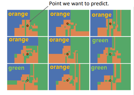
- 6 votes orange : 3 votes green \(\Rightarrow\) ORANGE
Bagging
- Bootstrap AGGregatING
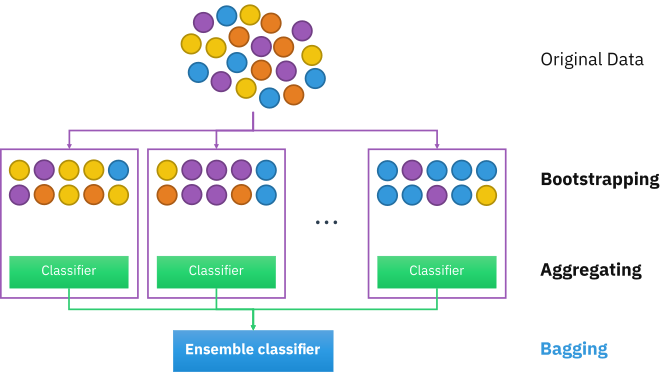
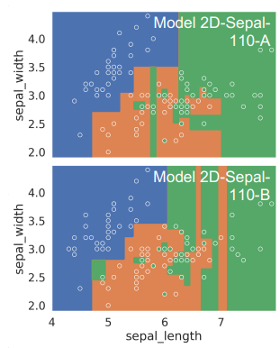
- but bagging not enough to reduce model variance
- decision trees look very similar to each other
-
one strong feature always used for first split 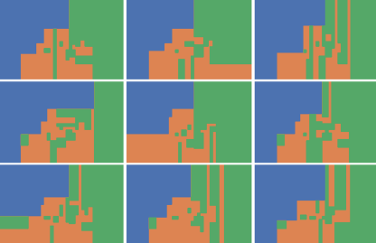
- \(\Rightarrow\) only use a sample of \(m\) features at each split
- usually \(m=\sqrt{p}\) for decision trees in classification (\(p\): # of features)
Random Forest Algorithm
- 2 hyperparameters: T and \(m\)
1. Bootstrap training data 'T' times. Fit decision tree each resample by:
  - start with data in one node (until all nodes are pure)
  - pick impure node
  - pick random subset of 'm' features
    → pick best feature 'x' and split value β  so that split loss is minimized
    (ex: x = petal_width, β = 0.8 => L=0.66)
  - split data into 2 nodes (x < β, x ≥ β)
2. [predict] ask T decision trees for prediction and take majority vote
- preventing growth, pruning, random forest \(\Rightarrow heuristics\)
- not provably best/mathematically optimal
- 그저 sounded good, implemented, worked well
- Why we use Random Forests
- Versatile (regression & classification 가능)
- Invariant to feature scaling and translation
- Automatic feature selection
- nonlinear decision boundaries without complicated feature engineering
- 다른 nonlinear model보다 overfit 심하진 않음
- Example of ensemble method: combine knowledge of many simple models to create sophisticated model
- Example of bootstrap: reduce model variance
- Provide alternate non-linear framework for classification & regression
- overfitting probability high
- boundaries can be more complex
- underlying principle fundamentally different