Keras Programming
in Notes / Artificialintelligence / Introductiontoai
DAY 7 - 9
- Keras
- MNIST Data Set
- Linear Regression Implementation
- Binary Classification Implementation
- Softmax Classification Implementation
- ANN implementation
Keras
- Keras Neural Networks:
- if hidden layer eliminated, changed into other pure classifications (binary, softmax, etc)
- if pure (without hidden layers) show better accuracy => Don’t use hidden layers
Keras Tips :
[activation] setting in
[Dense] keras.layers in
[add] function[loss] setting in
[compile] functionLinear Regression mse(mean squre error)Binary Classification sigmoid binary_crossentropySoftmax Classification softmax categorical_crossentropy- Disadvanatages of Keras : no control (modifications) of layers (only add)
- academics => PyTorch
- industry => Keras (quick to implememnt, simple)
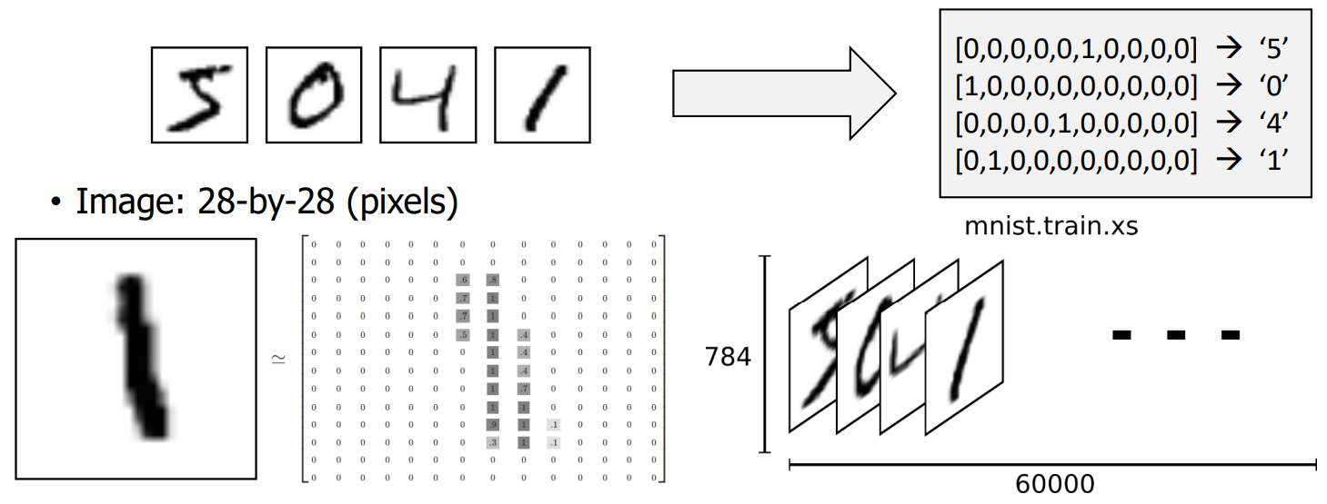
MNIST Data Set
- Hand-written images and their labels
- For training : 60,000
- For Testing : 10,000
- Image : 28 - by 28 (pixels)
- Neural Network Characteristics:
Compression Impact :- ex) 784 size input -> hidden layer with 1 unit
- => 784 unit compressed into 1 unit => loss of information on features
=> IF YOU DON’T HAVE MUCH INFORMATION ABOUT YOUR INPUT, MAINTAIN AS MUCH AS POSSIBLE DURING HIDDEN LAYER
- Mnist Data Set 특징: compression is pretty Okay because
- Simple
- Black-and-white
- Content is centered
Linear Regression Implementation
import numpy as np
import matplotlib.pyplot as plt
from keras.models import Sequential
from keras.layers import Dense
# Data
x_data = np.array([[1], [2], [3]])
y_data = np.array([[1], [2], [3]])
#Model, Cost, Train
model = Sequential()
model.add(Dense(1, input_dim=1 )) # 1 output only
model.compile(loss = 'mse', optimizer = 'adam') # adam | sgd (up to you)
model.fit(x_data, y_data, epochs= 1000, verbose = 0)
model.summary()
# Infernece
print(model.get_weights())
print(model.predict(np.array([4]))) # 4 expected
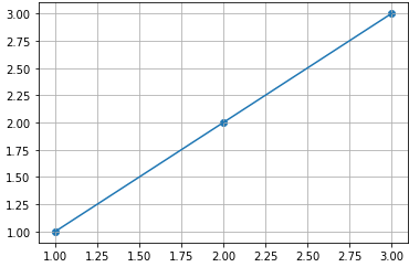
#Plot
plt.scatter(x_data, y_data)
plt.plot(x_data, y_data)
plt.grid(True)
plt.show()
- Summary Output
Model: "sequential" _________________________________________________________________ Layer (type) Output Shape Param # ================================================================= dense (Dense) (None, 1) 2 [W = 1 + b = 1] ================================================================= Total params: 2 Trainable params: 2 Non-trainable params: 0 _________________________________________________________________ - Inference Output
[array([[1.1798639]], dtype=float32), array([-0.38375837], dtype=float32)] 1/1 [==============================] - 0s 53ms/step [[4.335697]] => almost '4' => Correct - Plot Output
Binary Classification Implementation
import numpy as np
from keras.models import Sequential
from keras.layers import Dense

# Data
x_data = np.array([[1, 2], [2, 3], [3, 1], [4,3], [5, 3], [6, 2]])
y_data = np.array([[0], [0], [0], [1], [1], [1]])

#Model, Cost, Train
model = Sequential()
model.add(Dense(1, activation='sigmoid')) # Just 1 classification (0 또는 1)
model.compile(loss = 'binary_crossentropy', optimizer = 'sgd', metrics=['accuracy'])
model.fit(x_data, y_data, epochs= 10000, verbose = 1)
model.summary()

# Infernece
print(model.get_weights())
print(model.predict(x_data))
- Model Output
Model: "sequential" _________________________________________________________________ Layer (type) Output Shape Param # ================================================================= dense (Dense) (None, 1) 3 [W = 2 + b = 1] ================================================================= Total params: 3 Trainable params: 3 Non-trainable params: 0 _________________________________________________________________ - Inference Output
[array([[1.4749366 ],
     [0.31867325]], dtype=float32), array([-5.576844], dtype=float32)]
1/1 [==============================] - 0s 70ms/step
[[0.03033758] => 0
[0.15829739]  => 0
[0.30293486]  => 0
[0.78226626]  => 1
[0.94013095]  => 1
[0.98035556]] => 1  => Same with out sample data (y_data)
Softmax Classification Implementation
import numpy as np
from keras.models import Sequential
from keras.layers import Dense

# Data
x_data = np.array([[1,2,1,1], [3,1,3,4], [4,1,5,5], [1,7,5,5], [1,2,5,6], [1,6,6,6], [1,7,7,7]])

y_data = np.array([[0,0,1], [0,0,1], [0,1,0], [0,1,0], [0,1,0], [1,0,0], [1,0,0]]) # 3 Classifications possible

# Model, Cost

model = Sequential()
model.add(Dense(3, activation='softmax')) # units=3 cuz 3 classifications
model.compile(loss = 'categorical_crossentropy', optimizer = 'sgd', metrics=['accuracy'])

# Training
model.fit(x_data, y_data, epochs = 10000, verbose = 1)
model.summary()

# Inference
y_predict = model.predict(np.array([[1,11,7,9]]))
print(y_predict)
print('argmax : ', np.argmax(y_predict)) # returns index of max value
ANN implementation
from keras.utils import np_utils
from keras.datasets import mnist
from keras.models import Sequential
from keras.layers import Dense

#MNIST data

# 28*28*60,000; 60,000 numbers;  28*28*10,000; 10,000 numbers
(train_images, train_labels), (test_images, test_labels) = mnist.load_data()
#Check Shape
print(train_images.shape, train_labels.shape, test_images.shape, test_labels.shape)

# Change Shape 3D (28*28*60,000) -> 2D (60,000 * 784)
# and change float
train_images = train_images.reshape(train_images.shape[0], 784).astype('float32')/255.0
# Change value (10,000 , ) -> (10,000 * 10)
# for number of classifications and change float
test_images = test_images.reshape(test_images.shape[0], 784).astype('float32')/255.0

train_labels = np_utils.to_categorical(train_labels) # One-Hot Encoding
test_labels = np_utils.to_categorical(test_labels) # One-Hot Encoding

print(train_images.shape, train_labels.shape, test_images.shape, test_labels.shape)

# Model

model = Sequential()
model.add(Dense(256, activation='relu')) # Hidden Layer #1: units=256, activation = 'relu'
model.add(Dense(256, activation='relu')) # units=256, activation = 'relu'
model.add(Dense(256, activation='relu')) # units=256, activation = 'relu'
model.add(Dense(10, activation='softmax')) # Output Layer: Distinguish between numbers 0 ~ 9

# Cost (Loss) Function binary 아닌 categorical, Soft Gradient Descent
model.compile(loss = 'categorical_crossentropy', optimizer = 'sgd', metrics=['accuracy'])

#Training
model.fit(train_images,
          train_labels,
          epochs = 5,    #iterations: 5 times (5 * 60,000 data)
          batch_size=32, # (5*60000) = 300,000 data divided by batch_size for input
          verbose = 1)   # verbose = 1 : see intermediate results
                         # verbose = 0 : don't see 중간 결과

#Testing (the test images provided by Mnist)
cost, accuracy = model.evaluate(test_images, test_labels)

print('Accuracy: ', accuracy)
model.summary()
- Testing Output (verbose, by Epoch)
Epoch 1/5
1875/1875 [==============================] - 11s 6ms/step - loss: 0.6092 - accuracy: 0.8393
Epoch 2/5
1875/1875 [==============================] - 11s 6ms/step - loss: 0.2518 - accuracy: 0.9267
Epoch 3/5
1875/1875 [==============================] - 11s 6ms/step - loss: 0.1945 - accuracy: 0.9441
Epoch 4/5
1875/1875 [==============================] - 10s 6ms/step - loss: 0.1592 - accuracy: 0.9543
Epoch 5/5
1875/1875 [==============================] - 11s 6ms/step - loss: 0.1347 - accuracy: 0.9602
313/313 [==============================] - 1s 3ms/step - loss: 0.1313 - accuracy: 0.9608
Accuracy Increases => final accuracy = 96%- sometimes when testing with real values, the accuracy is lower than the training accuracy.
- reason => Test Data and Training Data differs a lot
Summary Output (verbose, by Epoch)
Model: "sequential_7" _________________________________________________________________ Layer (type) Output Shape Param # [W + b] ================================================================= dense_25 (Dense) (None, 256) 200960 [(786*256) + 256] dense_26 (Dense) (None, 256) 65792 [(256*256) + 256] dense_27 (Dense) (None, 256) 65792 [(256*256) + 256] dense_28 (Dense) (None, 10) 2570 [(256*10) + 10] ================================================================= Total params: 335,114 [전체 합] Trainable params: 335,114 Non-trainable params: 0 _________________________________________________________________- One Hot Encoding
- 1의 위치에 따라서 labeling
- ex) [ 1, 0, 0, 0, 0 …] => 0
- in case of softmax => Number of outputs = Number of classifications